Tempas オプションモジュール

• Object and Exit Wave Reconstruction Package
  (オブジェクトおよび波面(Exit Wave)の再構築パッケージ)
  
• Scripting Package
  (スクリプティング・パッケージ）

Object and Exit Wave Reconstruction Package

オブジェクトおよび波面(Exit Wave)の再構築パッケージ

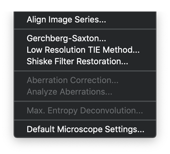
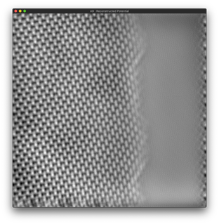
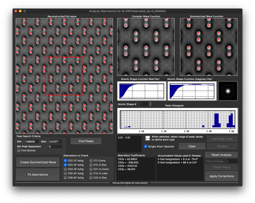
再構成ソフトウェアパッケージは、波面 (Exit Wave) 関数 (波動関数) と、焦点移動 (thru-focus-series) 、および、収差補正位相プレート、画像の整列、Shiske フィルタによるオブジェクトの復元をもとに標本ポテンシャルを求める各種アルゴリズムで構成されています。現在実装されている機能を以下に示します：

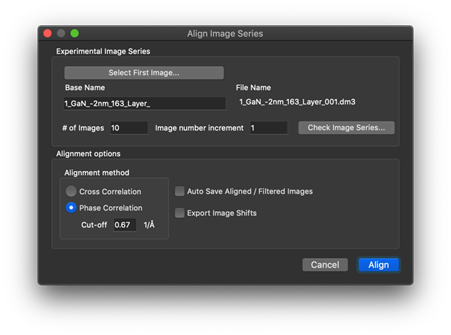
• 相互相関 (cross correlation) または位相相関 (phase correlation) を使用した系列画像の整列
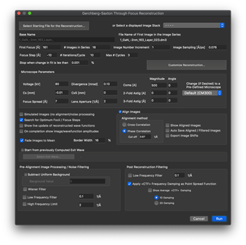
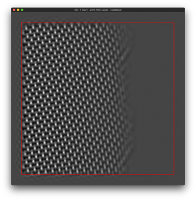
• Gerchberg-Saxton アルゴリズムによる波面 (exit wave) の回復
• 低解像度トランスポートによる波面強度の再構築
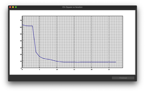
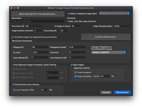
• Shiske フィルタによるオブジェクトの復元
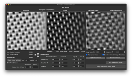
• 収差補正位相プレート (Aberration correcting phase plate)
• ガウスピークの当てはめに基づく収差分析
• 最大エントロピー法によるデコンボリューション (Maximum Entropy Deconvilution)

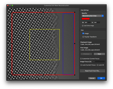
スクリーンショット例

Scripting Package

スクリプティング・パッケージ

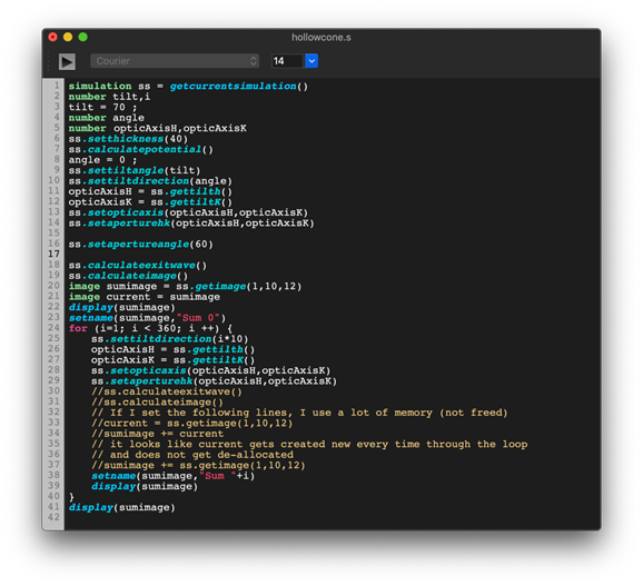
スクリプトの記述は、シミュレーション制御やイメージ処理を自動化することにより Tempas の機能を拡張する効果的な手段です。全く新しいアルゴリズムを作成してそれを試したり、様々なアイデアを実装することもできます。

Tempas のスクリプティング言語は、C, C++ によるプログラムの作成や、Digital Micrograph (copyright Gatan Inc.) 用のスクリプティング言語の経験のある方ならどなたでもすぐにご利用いただけます。このスクリプト言語には、Digital Micrograph のスクリプトを作成したことがある方のために、多くの DM スクリプトを殆ど修正なしで実行できる組み込み関数が用意されています。

最新のスクリプト言語のリファレンスマニュアルをダウンロードするには、こちらをクリックしてください。

▶コードを読みやすくするシンタックスカラーリング (構文の色分け) 機能と、操作性を向上するワード補完機能が追加されています

例: Digital Micrograph 互換スクリプト

・例1:

Image test = newimage(“test”,512,512)      // Creates a float image  of size 512 by 512
test = exp(-iradius*iradius/100)      // Fills the image with a gaussian with sigma = 10
display(test)      // Displays the image

・例1:DM とは互換性のない記述例

Image test(512,512,exp(-iradius**2/100))    
test.show()       // Displays the image

・例2:

Image test = newimage(“test”,512,512)      // Creates a float image  of size 512 by 512
test = sin(2*pi()*icol/8)+sin(2*pi()*irow/12)
                              // Fills the image with cross-fringes
                              // of period 8 and 12 pixels in x , y
display(test)      // Displays the image

・例2:DM とは互換性のない記述例

Image test(512,512,sin(2*pi*icol/8)+sin(2*pi*irow/12))     
test.display()       // Displays the image

・例3:

/ Precession Tilt series
// This is summing over the power-spectrum of the exit wave function
// by spinning the beam in a circle. The beam tilt is theta (30 mrad).
// The increment in the azimuthal angle is dphi (6 degrees)
// A table of HKL values for different thicknesses is shown
// For illustration purposes, a precession image is also calculated

number theta = 30 // The tilt angle in mrad
number phi = 0 // Tilt angle (degrees) with respect to a-axis
number dphi = 6 // increments in tilt angle (degrees)

simulation sim = getsimulation() // Get the simulation

// We are making sure that everything has been calculated and is current
sim.calculateall()

image xw = sim.loadexitwave() // Declare and load the exit wave
image im = sim. loadimage() // Declare and load the image
image sumim = im ; sumim = 0 ; // Declare the sum for the images and zero
image sumps = xw ; sumps = 0 ; // Declare the sum for the powerspectrum
// and zero

Openlogwindow()

for(number thickness = 10; thickness <= 100; thickness += 10) {
    sim.setthickness(thickness)
    number i = 0 // declare and  initialize our counter
    for(phi = 0 ; phi < 360; phi += dphi) { // loop over the azimuthal angle
        sim.settilt(theta,phi) // set the tilt of the specimen
        // this is equivalent to the tilting the beam
        sim.calculateexitwave() // Calculate the new exit wave
        sim.calculateimage() // Calculate the new image
        sumim += sim. loadimage() // Add the image to the sum
        xw = sim. loadexitwave() // Load the exit wave
        xw.fft() // Fourier transform to get the frequency
        // complex coefficients
        xw *= conjugate(xw) // Set the complex PowerSpectrum
        // If we had  used xw.ps() to get the
        // power spectrum we would have had a real
        // image in “real” space
        sumps += xw // Add the powerspectrum to the sum
        i++ // Keep track of the count
        print("phi = "+phi) // Just to know where we are in the loop
    }
    sumim /= i // Divide by the number of terms in the sum

    // Create a rectangular image of size 1024 by 1024 of sampling 0.1 Å (default) 
    image precessionImage = sim.createimage(sumim,1024)

    precessionImage.setname("Image Precession")
    precessionImage.show() // Show the summed images

    sumps /= i // Divide by the number of terms in the sum
    sumps.sqrt() // To compare with the Scattering factors

    // Create a rectangular image of size 1024 by 1024 out to gMax = 4 1/Å
    // with a convergence angle of 0.2 mrad
    image precessionPS = sim.createfrequencyimage(sumps,1024,0.2,4)
    precessionPS.setname("Power Spectrum Precession Thickness "+ sim.getthickness())

    precessionPS.show() // Show the summed power spectrum
    sumps.setname("thickness " + sim.getthickness())
    sim.createhkltable(sumps)
}