日本語
English
株式会社ヒューリンクス
TEL:03-5642-8385
営業時間:9:00-17:30
HRTEMの画像/回折シミュレーション機能
| ※ MacTempasXの後継品「Tempas」(macOSX/Windowsy用 64bit対応) がリリースされました。 ※ Apple社が32bit アプリケーションのサポートを終了しているため、旧製品MacTempasXは 開発終了となります。MacTempasXユーザの方の最新版ダウンロードはこちらをご覧ください。 |
「Tempas」は、HRTEM (高分解能透過電子顕微鏡) の画像/回折シミュレーション機能に加え、STEM (走査型透過電子顕微鏡) および CBED (収束電子回折) 計算機能を実装しています。画像の定量的な比較や構造精密化はもちろん、様々な機能を備えた前バージョン「MacTempas」のコードを完全に書き直したプログラムです。Tempas は開発プラットフォームに QT を利用していますので、macOS 版の開発と同時に Windows 版を作成することが可能となりました。
Tempas にはMacTempas の機能がそのまま維持されており、MacTempas の操作法を知っている方ならどなたでも Tempas を違和感なく操作できるはずです。さらに、グラフィカルユーザーインターフェース (GUI) が完全に書き換えられ、MacTempas には出来なかった機能が Tempas には追加されています。操作の多くは CPU のマルチコアを利用しているため、様々な操作がコア数に応じて高速化されます。
開発元:Total Resolution
機能一覧
Tempas の主な機能
- 完全なマルチスライス計算による高解像度 TEM 画像と動的回折パターン
- 完全なマルチスライス計算による高解像度 STEM 画像
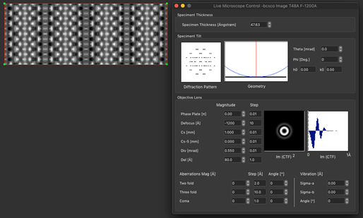
- 「ライブ」コントロールにより計算される HRTEM 画像とシミュレーションの各種パラメータの関数としての波面 (exit wave)
- 運動学的 SAD パターンと菊池パターンの計算
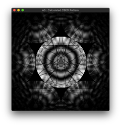
- 運動学的 CBED パターンの計算
- ブロッホ波計算による CBED パターン
- リングパターン
- 自動計算による HRTEM 連続傾斜像
- シミュレーション画像と実験画像の完全な定量的比較
- 画像の定量的照合に基づく構造および顕微鏡パラメータの精密化
- 逆空間テーブル、面間隔と角度の計算機
- 完全な画像操作
- 基本的画像処理全般
- 高度な画像処理機能、実空間、逆空間フィルタ、マスク、ノイズフィルタ等
- ピークの検出、ピークの当てはめ、および、格子のあてはめ
- パターン検索のためのテンプレートマッチング機能
- 実空間と逆空間の置き換えと歪み解析
- 結晶学的画像処理
- 回折パターンの定量化
- モチーフ抽出とノイズ推定による平均化
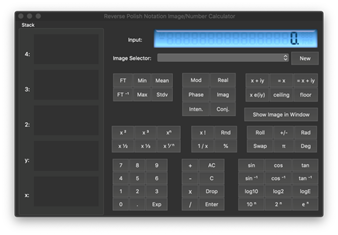
- 完全な逆ポーランド記法による画像計算機
- 画像の整列 (alignment)
- フォーカスの決定
- Gatan Digital Micrograph 画像 (画像データとカリブレーション) の読み込みのサポート
- オプション:Digital Micrograph 互換スクリプト言語
- オプション:波面 (exit wave) とオブジェクトの再構築パッケージ
- …上記の他にも多彩な機能が装備されています
Tempas オプションモジュール
- Object and Exit Wave Reconstruction Package
(オブジェクトおよび波面(Exit Wave)の再構築パッケージ) - Scripting Package
(スクリプティング・パッケージ)
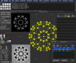
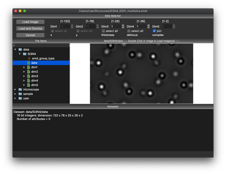
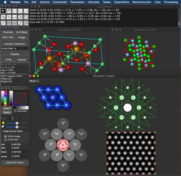
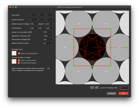
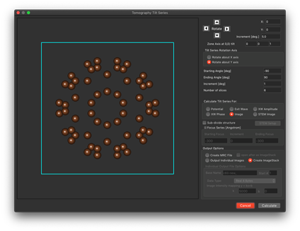
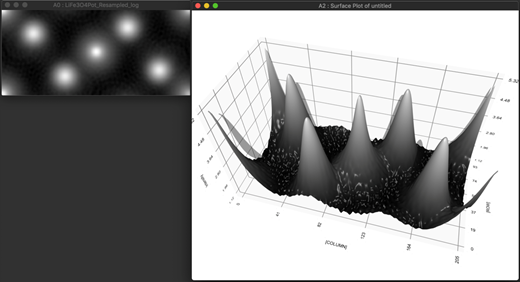
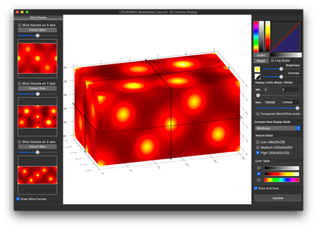
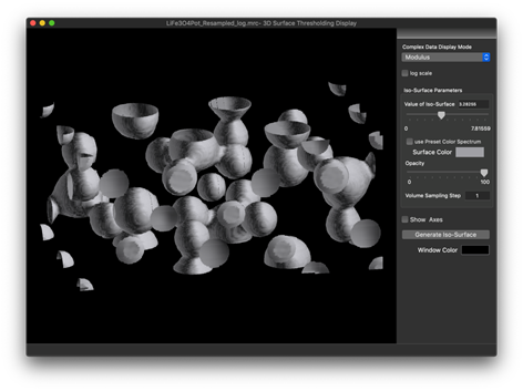
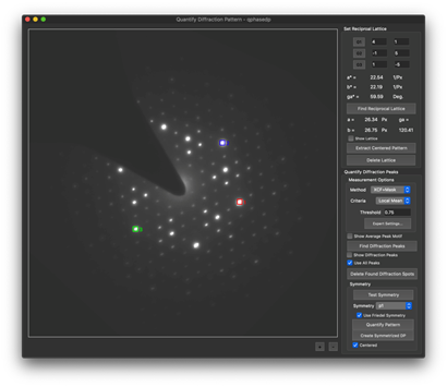
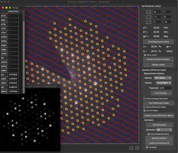
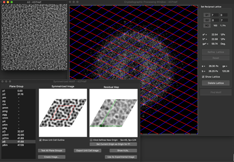
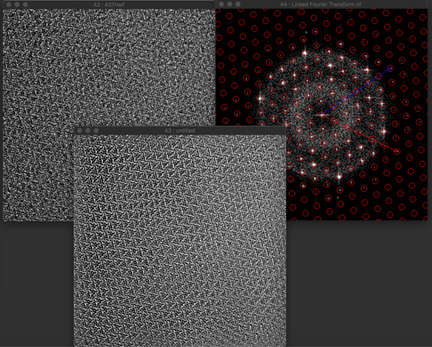
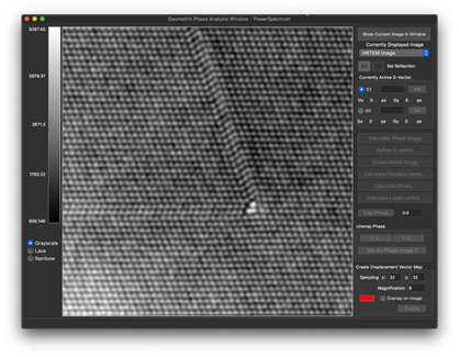
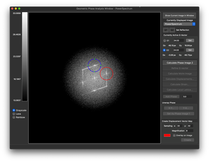
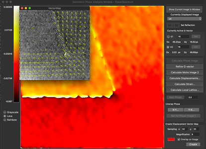
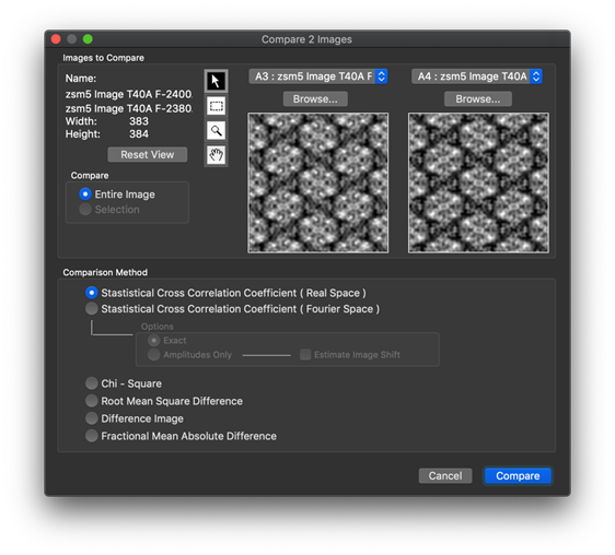
Tempas のスクリーンショット例

動作環境
動作環境
Tempas macOS 版
macOS 10.12 以降
Tempas Windows 版
Windows (64bit)
ライセンス
※ご購入後のダウンロード時にプラットフォームを選択いただきます。
どちらもご利用いただけますが同時起動はUSBキーで1ライセンスにつき1台になります
※製品は、英語版(英語PDFマニュアル付き)です
トライアル
デモ版お申込み
製品価格
※ 製品価格・アップグレード価格は、下記のお見積もりフォームよりお問合せください。
| ▼ハードウェアキーについて ・Tempas と CrystalKitXの両方を同時にご注文いただくと、ライセンス認証用のハードウェアキーが1本同梱されます。(同一PC上での使用を前提としています) ・Tempas / CrystalKitX をそれぞれ別のマシンでお使いになりたい場合は、お見積りご請求の際にお知らせください。 |
お見積り・ご購入
サポート
サポート情報 (旧製品MacTempasX関連含む)
- Tempas / CrystalKit アップデート情報 (2016/11/14) (17/01/23 )
- Tempas インストール手順 (17/01/23 )
- MacTempasX Ver2 の File メニューに、以下のコマンドが表示されません。(09/08/31 )
簡易操作マニュアル
(Tempasユーザも参考用に参照可)
最新版ダウンロード
最新版は下記よりダウンロードできます。
(旧製品MacTempasX用含む)アップデータおよびPDF マニュアル(英語・Tempasユーザも参照可)のダウンロード
- Software Updates (開発元)