|
| サイトマップ | |
||
|
| サイトマップ | |
||
応用分野においては、従属変数と1つ以上の独立変数を含む方程式で関数が間接的に (implicitly: 陰に) 定義されることがしばしばあります。関数 implicit を使えば、各独立変数の値を指定したときの従属変数についての方程式を解くことができます。
rv = implicit(expr, a, b, indvar, maxroots)
式 expr には、従属変数と独立変数が含まれます。方程式は、この式に = 0 を設定して定義します。式は、ユーザー定義関数である必要があります。
k(u,v) = u^2 – 3*u*v + v^2
このとき、解を求める方程式は、k(u,v) = 0 となります。この事例の場合、関数 implicit の最初の引数に k(u,v) を設定します。
従属変数 (solution variable) は常に、ユーザー定義関数の引数リストの最初の変数であるとみなされます。上記の例では、u がこの変数に相当します。
r(u,v,w) = (u+v*w)*exp(u*w)
この事例の場合、u が従属変数、v と w が独立変数です。
ユーザー定義関数には、引数リストにあるもの以外の変数も含まれている可能性がありますので、これらのパラメーターは、関数を定義する時点において割り当てた値であると考えます。いずれのパラメーターも、それぞれ単一の数値によって定義されたスカラー量であるということが重要です。パラメーターが範囲の場合は、その範囲の最初の値が使用されます。
引数 a と 引数 b は、解の探索を行う区間の左右それぞれの端点です。
引数 indvar は、独立変数の値を定義する式または記号で、方程式を解くために使用します。通常は、範囲で定義します。
x=col(1)
f=implicit(k(u,v),-10,10,x)
このトランスフォームは、列 1 から値をひとつ取り出し、それを変数 v に代入し、方程式 k(u,v)=0 を変数 u について解くものです。これを列1にある全ての値に対して繰り返します。結果は、変数 f に代入されます。
独立変数がユーザー定義関数に複数リストされている場合、関数に表れる順に独立変数の値が連結され、その結果が引数 indvar に代入されます。
implicit に2つの独立変数が使用されています:
x=col(1)
y=col(2)
k(u,v,w)=u^2+v^2+w
col(4)=implicit(k(u,v,w),-10,10,{x,y})
この事例の場合、列1から値をひとつ取り出して変数 v に代入し、同じ行の列2の値を変数 w に代入します。そして、変数 u について方程式 k(u,v,w) を解きます。この計算は、列1 と列 2 の入力値がなくなるまで繰り返されます。
ここで重要となるのは、引数 indvar にデータ範囲を指定する場合、そのデータは、方程式の独立変数の数だけ均等に配分される点です。データは最初の独立変数から順番に均等に分割され、それ以外の余りは関数 implicit では無視されます。例えば、引数 indvar に指定する範囲に値が 14 個あり、問題の中に独立変数が3つある場合、1~4 番目の値は最初の変数に、5~8 番目の値は第2の変数に、9~12 番目の値は第3の変数に割り当てられます。最後に余った2つの値は無視されます。
引数 maxroots はオプションの引数で、指定した独立変数の値の各セットを計算する従属変数の値の最大数を表します。デフォルトは 1 です。
戻り値 (Return Value)、すなわち、rv が、求められた解の全てのリストまたは範囲です。戻り値の数は、独立変数の値の各セットに対する引数 maxroots と常に等しくなります。
引数 maxroots の数を増やすと、規定区間における方程式のすべての解を求められる可能性が高くなります。また、関数 implicit の処理にかかる時間もそれだけ増加します。ある方程式の解を複数探索する場合、関数 implicit は、指定した区間を maxroots 分の等間隔の部分区間に区切ります。そして、部分区間のそれぞれから厳密に1つの解を探索します。結果として、その方程式に与えられた区間において maxroots で指定した数以上の解が実際にあったとしても、関数 implicit は、maxroots よりも少ない解を返します。方程式の区間 a と b におけるすべての解を求めるには、maxroots に (b - a)/delta よりも大きい値を設定するのが理想的です。ここで、delta は、すべての解に最も近い値を見積もります。
関数 implicit の出力は常にソートされ、引数 expr で指定した関数の根ごとに昇順で出力されます。
v について方程式 a*u^b/(c^b+u^b) - v =0 の解を求めます。結果は列1に代入されます。
a=95
b=3
c=1.5
x=data(0,10,.025)
k(u,v)=a*u^b/(c^b+u^b) - v
col(1)=implicit(k(u,v),0,10,x)
2つの変数をもつ陰関数の方程式をグラフ化するのは困難です。自明な方法は、独立変数として参照される1変数の値を幾つか選択し、従属変数となる残りの変数について方程式を解くことです。独立変数に与えられた値の範囲に関する方程式のグラフを完成させるには、その従属変数について方程式のすべて解を求める必要があります。
-5 ~ 5 の値をとる x について方程式 sin(x)^2 = y*(y-1)*(y-2) をグラフ化するとしましょう。この方程式の y の値が 0 より大きいことは明らかです。そうでなければ sin(x)^2 が負の値をとるなることになりますが、それはありえません。また、y の値が 3 より小さいことは間違いありません。なぜなら、方程式の右辺が 1 より大きくなり、sin(x)^2 の値の最大値である 1 を超えてしまうからです。従って、y の探索区間を 0~3 の間とすることにします。この方程式を見ると、右辺は三次多項式なので、x の各値に対して最大で 3つの y 値があることがわかります。このことをふまえて引数 maxroots には 3 を設定することもできるでしょう。しかし、上記の説明の通り、与えられた x 値についての解がどれくらい正解に近いかわからないので、ここではこの値を maxroots = 10 と高めに設定することにします。
x=data(-5,5,.005)
k(u,v)=u*(u-1)*(u-2)-sin(v)^2
col(2)=implicit(k(u,v),0,3,x,10)
for i=1 to size(x) do
for j = 1 to 10 do
cell(1,10*(i-1) + j) = x[i]
end for
end for
最初の行は、区間 -5~5 で独立変数の値をいくつかサンプリングします。2行目では、0 を設定することで方程式を成り立たせる式を定義します。3行目にある関数 implicit の呼び出しには、探索の区間と maxroots に関する内容が含まれます。x の各値についての全ての解は、関数 implicit が配置する出力法に従って連続して表示されます。トランスフォームの残りの行は、それらの解に対応する x データを同じ 10 個の値として繰り返すことでワークシートに配置します。期待する全ての値は最大で 3つであることから、関数 implicit の出力には欠損値が多数含まれることになる点にご注意ください。グラフ化する際、これらの欠損値は単に無視されます。
トランスフォームを実行する前に、角度の単位に radians (ラジアン) が選択されていることを確かめてください。トランスフォームを実行した後、XY Pair のデータ形式に対して列1と列2を選択した簡単な散布図を作成します。以下のグラフが得られます:
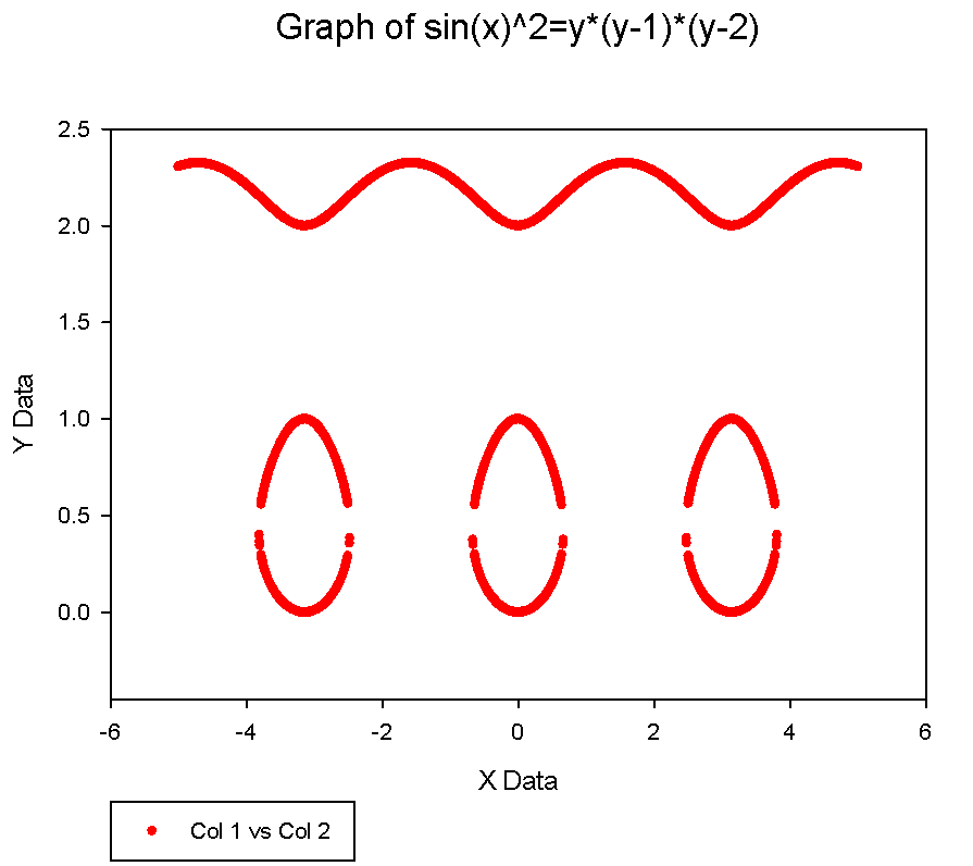
波状の曲線の下にあるほとんど閉じた 3つの曲線はぴったりと閉じられるべきですが、それにはより多くのサンプルポイントが必要となります。
この例は、フィッティングモデルを暗に定義するカーブフィットの方程式のテキストを示します。この特殊な例では、テーブル内のデータは、暗に定義される楕円によってあてはめられます。
|
|
関数 implicit をカーブフィッティングに用いる場合、解を一意に決定できる値であれば任意の値を maxroots に設定することができます。しかし、maxroots が 1 より大きい場合は、最初の根に1を設定する必要があります (もしくは、関数 implicit の呼び出しの後に単一の解を選ぶ方法を付けます)。そうでないと、戻り値は独立変数の値と正確に一致しません。
In applications, a function is often defined implicitly by an equation involving a dependent variable and one or more independent variables. Use the implicit function to solve the equation for the dependent variable when a value for each independent variable has been specified.
rv = implicit(expr, a, b, indvar, maxroots)
The expression expr contains the dependent variable and the independent variables. The equation is defined by setting this expression equal to zero. The expression must be a user-defined function. For example, the user-defined function might be:
k(u,v) = u^2 – 3*u*v + v^2
and the equation being solved becomes k(u,v) = 0. In this case, you would set the first argument in the implicit function to k(u,v).
It is assumed that the dependent variable (the solution variable) is always the first variable in the argument list of the user-defined function. In the above example, this variable is u.
The argument list can have any number of independent variables, such as:
r(u,v,w) = (u+v*w)*exp(u*w)
In this case, u is the dependent variable with v and w as the independent variables.
The user-defined function may contain other variables than those in its argument list. These parameters are assumed to have assigned values when the function is defined. It is important that each parameter be a scalar quantity defined by a single numeric value. If any parameter is a range, then only the first value in that range is used.
a and b are the left and right endpoints, respectively, of the interval over which the solution search for the dependent variable takes place.
indvar is an expression or symbol that defines the values of the independent variables that are used to solve the equation. It is usually defined by some range. For example, suppose we have transform:
x=col(1)
f=implicit(k(u,v),-10,10,x)
Then this transform takes a value from column 1, assigns it to the variable v, and solves the equation k(u,v)=0 for the variable u. This is then repeated until all values in column 1 have been used. The results are then assigned to the variable f.
If more than one independent variable is listed in the user-defined function, then the values of the independent variables are concatenated in the order they appear in the function and the result is assigned to indvar. For example, in the transform below we have the implicit function used with two independent variables:
x=col(1)
y=col(2)
k(u,v,w)=u^2+v^2+w
col(4)=implicit(k(u,v,w),-10,10,{x,y})
In this example, a value from column 1 is assigned to the variable v and a value for column 2, in the same row, is assigned to variable w. The equation k(u,v,w) is then solved for the variable u. This process is repeated until there are no more entries in columns 1 and 2.
It is important to note that when a range of data is provided to the argument indvar, then that data is divided equally among the independent variables in the equation. The data will be partitioned this way, beginning with the first independent variable, and the implicit function will ignore the remainder. For example, if indvar is provided a range of 14 values and there are 3 independent variables in the problem, then the values 1-4 will be assigned to the first variable, values 5-8 will be assigned to the second variable, and values 9-12 will be assigned to the third variable. The last two values will be ignored.
maxroots is an optional argument, representing the maximum number of dependent variable values to compute for each specified set of values of the independent variables. The default value is 1.
The Return Value, or rv, is the list or range of all of the solutions that were found. The number of values returned will always be equal to maxroots for each set of independent variable values. If fewer roots than maxroots are found, then the remaining values returned will be missing values. The reason for inserting the missing values is so the output of the different functions can be distinguished.
This first example finds a solution of the equation a*u^b/(c^b+u^b) - v =0 for each value of v in the sampled data from the interval from 0 to 10. The results are written to column 1.
a=95
b=3
c=1.5
x=data(0,10,.025)
k(u,v)=a*u^b/(c^b+u^b) - v
col(1)=implicit(k(u,v),0,10,x)
Graphing an implicit equation with two variables can be difficult. The obvious way is to select several values of one variable, which will be referred to as the independent variable, and solve the equation for the remaining variable, which will be the dependent variable. In order to get the complete graph of the equation over a given range of values for the independent variable, we need to obtain all of the solutions of the equation for the dependent variable.
Suppose we wish to graph the equation sin(x)^2 = y*(y-1)*(y-2) for values of x between -5 and 5. It is clear that the y values for this equation must be greater than 0, otherwise sin(x)^2 would be negative, which is impossible. Also, any y value must be less than 3, otherwise the right side of the equation would be greater than 1, which is the largest value of sin(x)^2. Thus, we will choose our search interval for y between 0 and 3. Looking at the equation, we see that for each value of x there are at most 3 values of y since the right side of the equation is a cubic polynomial. Knowing this, we could set maxroots equal to 3. However, from the discussion in the remarks above, since we don’t know how close the solutions are for a given x value, we will set this value higher to maxroots = 10.
The transform below generates the data that will be used to obtain the graph.
x=data(-5,5,.005)
k(u,v)=u*(u-1)*(u-2)-sin(v)^2
col(2)=implicit(k(u,v),0,3,x,10)
for i=1 to size(x) do
for j = 1 to 10 do
cell(1,10*(i-1) + j) = x[i]
end for
end for
The first line samples several values of the independent variable over the interval from -5 to 5. The second line defines the expression that will be set to zero to give us the equation. The call to the implicit function in the third line contains our information for the search interval and maxroots. Because of how the implicit function arranges the output, with all solutions for each x-value displayed consecutively, the remaining lines of the transform arrange our x-data in the worksheet by repeating a value for the 10 corresponding solutions. Note that there will be many missing values in the output of the implicit function since we know that a maximum of three values is all we expect. When graphing, these missing values will simply be ignored. Before running the transform, make sure that radians is selected as the angular units.
After running the transform, create a simple scatter plot with columns 1 and 2 selected for the XY Pair data format. The resulting graph is:
The three nearly closed curves below the undulating curve should indeed be closed, but more sampled points are needed.
This example shows the equation text for a curve fit in which the fit model is defined implicitly. In this particular example, the data in the table is fit by an ellipse that is defined implicitly.
| -2.0000 | 0.1000 | [Variables] | |
| -1.5000 | 0.3000 | x=col(1) | |
| -1.0000 | 0.4000 | y=col(2) | |
| -0.5000 | 0.6000 | [Parameters] | |
| 0.0000 | 0.5000 | a = .01 | |
| 0.5000 | 0.6000 | b = .01 | |
| 1.0000 | 0.5000 | [Equation] | |
| 1.5000 | 0.2500 | k(u,v)=a*v^2+b*u^2-1 | |
| 2.0000 | 0.1000 | f=implicit(k(u,v),0,10,x) fit f to y [Constraints] a>0 b>0 [Options] tolerance=1e-010 stepsize=1 iterations=200 |
When using the implicit function in curve fitting, you can set the value of maxroots to any value which is sufficient to locate one solution. However, if maxroots is greater than 1, you must set the value of firstroot to 1 (or follow the call of the implicit function with a method of selecting one solution), for otherwise the returned values cannot be properly matched to the independent variable values.