PyTecplot サンプルスクリプト

オリジナルサイト：https://github.com/Tecplot/handyscripts/tree/master/python

• スクリプトを実行するには
• 00_hello_world.py
• 01_load_layout_save_image.py
• 03_slices_along_wing.py
• 07_execute_equation.py
• 08_save_data.py
• 10_contour_filtering.py
• 11_linemaps.py
• 12_slices.py
• 14_isosurface.py
• 15_wing_mach_iso.py
• 17_streamtrace_line.py
• 19_streamtrace_2D.py
• 20_legend_line.py
• 22_view_3D.py
• 24_frame_position.py
• filledlines.py
• Forces_Moments_VS_Span.py
• Histogram.py
• UniformVectorViaGeom.py
• plot_max_over_time.py
• pyqt5_execute_macro_command.py

 

Tecplot をインストールしたディレクトリの pytecplot には多数のサンプルスクリプトが用意されています。また、下記の URL からもスクリプトを入手できます。

• https://github.com/Tecplot/handyscripts/tree/master/python/examples

 

スクリプトを実行するには

スクリプトを実行するには、 Tecplot 360 のポート 7600 との接続を確立するために "-c" オプションを付けてください。

• 例：

  py "C:\Program Files\Tecplot\...\examples\00_hello_world.py" -c

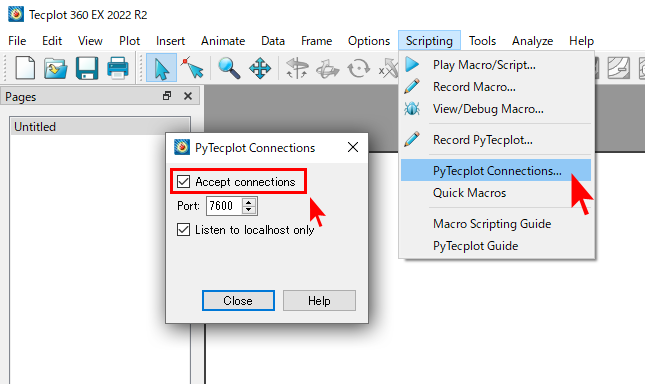
また、Tecplot 側で接続を有効にするために、Tecplot の Scripting メニューから PyTecplot Connections... を選択して、Accept connections にチェックを入れてください。

 

00_hello_world.py

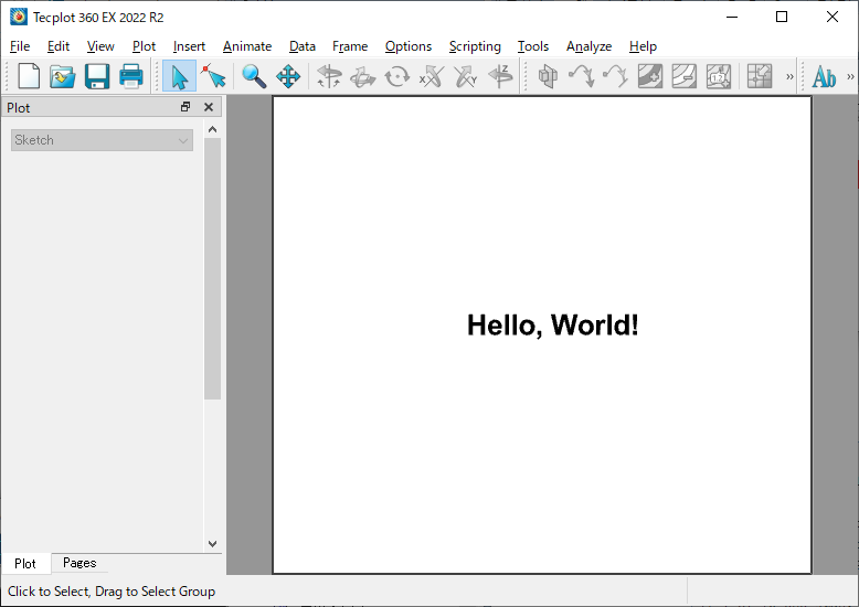
Tecplot の新規フレームに "Hello, world!" という文字を出力します。出力する文字には位置情報、フォントサイズを指定します。フレームと同じ内容の画像を PNG 形式で出力します。

• スクリプト：

  import logging
  logging.basicConfig(level=logging.DEBUG)
  import tecplot
  
  # Run this script with "-c" to connect to  Tecplot 360 on port 7600
  # To enable connections in Tecplot 360, click on:
  #   "Scripting" -> "PyTecplot  Connections..." -> "Accept connections"
  import sys
  if '-c' in sys.argv:
      tecplot.session.connect()
  
  tecplot.new_layout()
  
  frame = tecplot.active_frame()
  frame.add_text('Hello, World!', position=(36, 50), size=34)
  tecplot.export.save_png('hello_world.png', 600, supersample=3)

• 実行結果：
  

 

01_load_layout_save_image.py

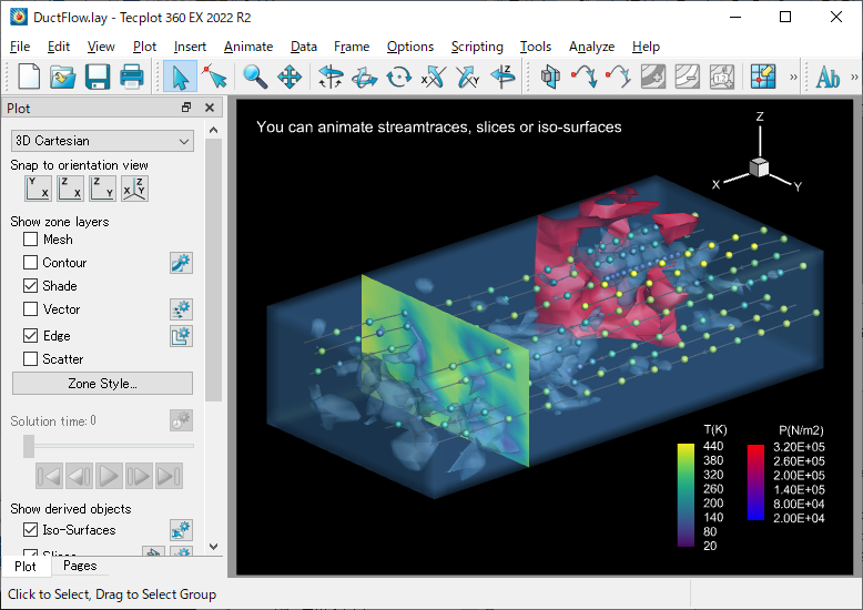
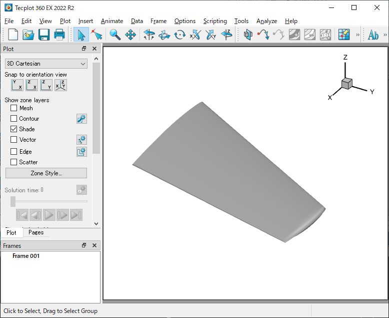
Tecplot の examples\SimpleData ディレクトリにあるレイアウトファイル DuctFlow.lay を読み込んで、同じ内容の画像を PNG 形式で出力します。

• スクリプト：

  import logging
  import os
  import sys
  
  logging.basicConfig(stream=sys.stdout, level=logging.INFO)
  
  import tecplot
  
  # Run this script with "-c" to connect to  Tecplot 360 on port 7600
  # To enable connections in Tecplot 360, click on:
  #   "Scripting" -> "PyTecplot  Connections..." -> "Accept connections"
  import sys
  if '-c' in sys.argv:
      tecplot.session.connect()
  
  examples_dir = tecplot.session.tecplot_examples_directory()
  infile = os.path.join(examples_dir, 'SimpleData', 'DuctFlow.lay')
  
  tecplot.load_layout(infile)
  tecplot.export.save_png('layout_example.png', 600, supersample=3) 
  

• 実行結果
  

 

03_slices_along_wing.py

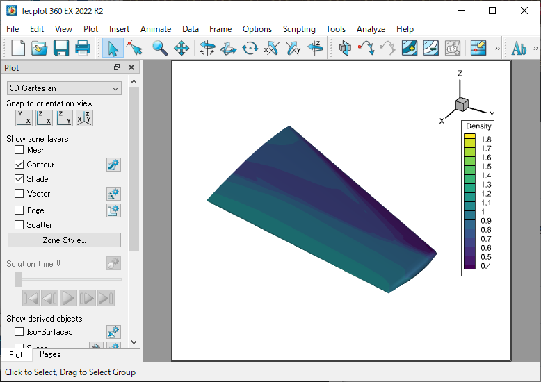
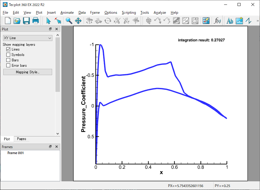
Tecplot の examples\OneraM6wing ディレクトリにあるレイアウトファイル OneraM6_SU2_RANS.plt を読み込んで、同じ内容の画像を PNG 形式で出力します。その後、翼のサーフェスデータから任意のスライスを抽出し、x 値を配列として取得したあと、正規化を行ないます。正規化されたスライス値を積分します。ここで、CFDAnalyzer を使って積分計算を行うためにインデックスの開始を１に指定します。フレームの aux データから積分結果を取得し、その結果をプロットの右上に配置します。linemap プロットのスタイルを設定して、データが表示されるように軸の範囲を調整します。最後に x/c の関数としてあらわされる圧力係数の画像をエクスポートします。

• スクリプト：

  import os
  import sys
  import logging
  
  logging.basicConfig(stream=sys.stdout, level=logging.INFO)
  
  import tecplot
  
  # Run this script with "-c" to connect to  Tecplot 360 on port 7600
  # To enable connections in Tecplot 360, click on:
  #   "Scripting" -> "PyTecplot  Connections..." -> "Accept connections"
  import sys
  if '-c' in sys.argv:
      tecplot.session.connect()
  
  examples_dir = tecplot.session.tecplot_examples_directory()
  datafile = os.path.join(examples_dir, 'OneraM6wing', 'OneraM6_SU2_RANS.plt')
  dataset = tecplot.data.load_tecplot(datafile)
  
  frame = tecplot.active_frame()
  frame.plot_type = tecplot.constant.PlotType.Cartesian3D
  frame.plot().show_contour = True
  
  # ensure consistent output between interactive  (connected) and batch
  frame.plot().contour(0).levels.reset_to_nice()
  
  # export image of wing
  tecplot.export.save_png('wing.png', 600, supersample=3)
  
  # extract an arbitrary slice from the surface data on  the wing
  extracted_slice = tecplot.data.extract.extract_slice(
      origin=(0, 0.25, 0),
      normal=(0, 1, 0),
      source=tecplot.constant.SliceSource.SurfaceZones,
      dataset=dataset)
  
  extracted_slice.name = 'Quarter-chord C_p'
  
  # get x from slice
  extracted_x = extracted_slice.values('x')
  
  # copy of data as a numpy array
  x = extracted_x.as_numpy_array()
  
  # normalize x
  xc = (x - x.min()) / (x.max() - x.min())
  extracted_x[:] = xc
  
  # switch plot type in current frame
  frame.plot_type = tecplot.constant.PlotType.XYLine
  plot = frame.plot()
  
  # clear plot
  plot.delete_linemaps()
  
  # create line plot from extracted zone data
  cp_linemap = plot.add_linemap(
      name=extracted_slice.name,
      zone=extracted_slice,
      x=dataset.variable('x'),
      y=dataset.variable('Pressure_Coefficient'))
  
  # integrate over the normalized extracted slice  values
  # notice we have to convert zero-based index to one-based  for CFDAnalyzer
  tecplot.macro.execute_extended_command('CFDAnalyzer4', '''
      Integrate
      VariableOption='Average'
      XOrigin=0 YOrigin=0
      ScalarVar={scalar_var}
      XVariable=1
  '''.format(scalar_var=dataset.variable('Pressure_Coefficient').index + 1))
  
  # get integral result from Frame's aux data
  total = float(frame.aux_data['CFDA.INTEGRATION_TOTAL'])
  
  # overlay result on plot in upper right corner
  frame.add_text('integration result: {:.5f}'.format(total), (60,90))
  
  # set style of linemap plot
  cp_linemap.line.color = tecplot.constant.Color.Blue
  cp_linemap.line.line_thickness = 0.8
  cp_linemap.y_axis.reverse = True
  
  # update axes limits to show data
  plot.view.fit()
  
  # export image of pressure coefficient as a function  of x/c
  tecplot.export.save_png('wing_pressure_coefficient.png', 600, supersample=3) 
  

• 実行結果
  
  

 

07_execute_equation.py

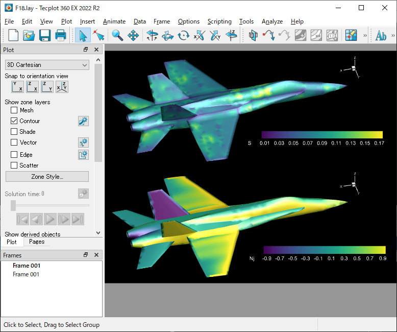
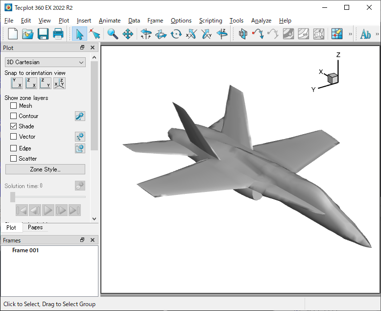
Tecplot の examples\SimpleData ディレクトリにあるレイアウトファイル F18.lay を読み込んで、同じ内容の画像を PNG 形式で出力します。データセットの Right Wing と Left Wing の２つの Zone の変数 Nj を変更します。この簡単な例では Nj を 10倍に変更します。変更後の結果を PNG 形式で出力します。

• スクリプト：

  import os
  import tecplot
  
  # Run this script with "-c" to connect to  Tecplot 360 on port 7600
  # To enable connections in Tecplot 360, click on:
  #   "Scripting" -> "PyTecplot  Connections..." -> "Accept connections"
  import sys
  if '-c' in sys.argv:
      tecplot.session.connect()
  
  examples_dir = tecplot.session.tecplot_examples_directory()
  infile = os.path.join(examples_dir, 'SimpleData', 'F18.lay')
  
  # Load a stylized layout where the contour variable  is set to 'Nj'
  tecplot.load_layout(infile)
  current_dataset = tecplot.active_frame().dataset
  
  # export original image
  tecplot.export.save_png('F18_orig.png', 600, supersample=3)
  
  # alter variable 'Nj' for the the two wing zones in  the dataset
  # In this simple example, just multiply it by 10.
  tecplot.data.operate.execute_equation('{Nj}={Nj}*10',
      zones=[current_dataset.zone('right  wing'),
             current_dataset.zone('left wing')])
  
  # The contour color of the wings in the exported  image will now be
  # red, since we have altered the 'Nj' variable by  multiplying it by 10.
  tecplot.export.save_png('F18_altered.png', 600, supersample=3) 

• 実行結果
  

 

08_save_data.py

Tecplot の examples ディレクトリにあるプロットファイル OneraM6wing\'OneraM6_SU2_RANS.plt を読み込みます。読み込んだファイルの 'WingSurface' Zone を PLT ファイルと ASCII ファイル (dat) に書き出します。

• スクリプト：

  from os import path
  import tecplot
  
  # Run this script with "-c" to connect to  Tecplot 360 on port 7600
  # To enable connections in Tecplot 360, click on:
  #   "Scripting" -> "PyTecplot  Connections..." -> "Accept connections"
  import sys
  if '-c' in sys.argv:
      tecplot.session.connect()
  
  examples_directory = tecplot.session.tecplot_examples_directory()
  infile = path.join(examples_directory, 'OneraM6wing', 
  'OneraM6_SU2_RANS.plt')
  dataset = tecplot.data.load_tecplot(infile)
  
  variables_to_save = [dataset.variable(V)
                       for V in ('x', 'y', 'z', 'Pressure_Coefficient')]
  
  zone_to_save = [dataset.zone('WingSurface')]
  
  # write data out to a binary PLT file
  tecplot.data.save_tecplot_plt('wing.plt', dataset=dataset,
                                 variables=variables_to_save,
                                 zones=zone_to_save)
  
  # write data out to an ascii file
  tecplot.data.save_tecplot_ascii('wing.dat', dataset=dataset,
                                   variables=variables_to_save,
                                   zones=zone_to_save) 

• 実行結果
  

 

10_contour_filtering.py

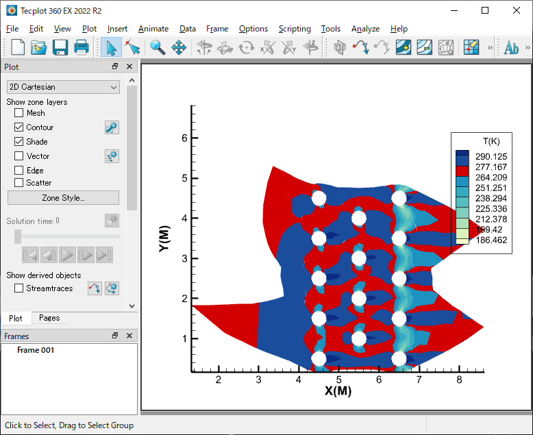
Tecplot の examples\SimpleData ディレクトリにあるプロットファイル HeatExchanger.plt を読み込みます。読み込んだプロットのタイプを 2D field Plot に設定します。boundary faces と contour を表示します。デフォルトでは、contour 0 が表示されます。contour の変数、カラーマップ、レベル数を設定します。contour のカラーマップを有効にします。この等高線のカラーマップの override を有効にします。override 0 を有効にし、1番目～4番目までのレベルに赤を設定します。得られた画像を PNG ファイルに出力します。

• スクリプト：

  from os import path
  import tecplot as tp
  from tecplot.constant import *
  
  # Run this script with "-c" to connect to  Tecplot 360 on port 7600
  # To enable connections in Tecplot 360, click on:
  #   "Scripting" -> "PyTecplot  Connections..." -> "Accept connections"
  import sys
  if '-c' in sys.argv:
      tp.session.connect()
  
  # load the data
  examples_dir = tp.session.tecplot_examples_directory()
  datafile = path.join(examples_dir, 'SimpleData', 'HeatExchanger.plt')
  dataset = tp.data.load_tecplot(datafile)
  
  # set plot type to 2D field plot
  frame = tp.active_frame()
  frame.plot_type = PlotType.Cartesian2D
  plot = frame.plot()
  
  # show boundary faces and contours
  surfaces = plot.fieldmap(0).surfaces
  surfaces.surfaces_to_plot = SurfacesToPlot.BoundaryFaces
  plot.show_contour = True
  
  # by default, contour 0 is the one that's shown,
  # set the contour's variable, colormap and number of  levels
  contour = plot.contour(0)
  contour.variable = dataset.variable('T(K)')
  contour.colormap_name = 'Sequential -  Yellow/Green/Blue'
  contour.levels.reset(9)
  
  # turn on colormap overrides for this contour
  contour_filter = contour.colormap_filter
  contour_filter.show_overrides = True
  
  # turn on override 0, coloring the first 4 levels red
  contour_override = contour_filter.override(0)
  contour_override.show = True
  contour_override.color = Color.Red
  contour_override.start_level = 7
  contour_override.end_level = 8
  
  # save image to file
  tp.export.save_png('contour_override.png', 600, supersample=3) 

• 実行結果
  

 

11_linemaps.py

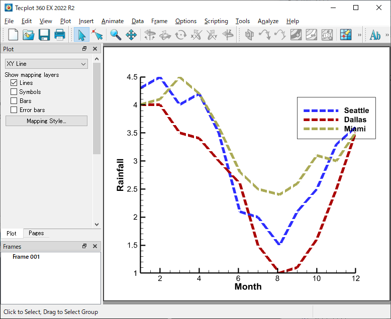
Tecplot の examples\SimpleData ディレクトリにあるデータファイル Rainfall.dat を読み込みます。アクティブなフレームを取得し、プロットタイプを XY Line に設定します。データセットの最初の 3 つのラインマップに名前、色、およびその他のいくつかのプロパティを設定します。３つのラインマップのそれぞれには roop を使って同じ設定を適用します。y 軸ラベルを設定します。凡例を有効にします。データ全体が表示されるよう軸の範囲を調整します。画像を PNG ファイルに保存します。

• スクリプト：

  from os import path
  import tecplot as tp
  from tecplot.constant import PlotType, Color, LinePattern, AxisTitleMode
  
  # Run this script with "-c" to connect to  Tecplot 360 on port 7600
  # To enable connections in Tecplot 360, click on:
  #   "Scripting" -> "PyTecplot  Connections..." -> "Accept connections"
  import sys
  if '-c' in sys.argv:
      tp.session.connect()
  
  # load data from examples directory
  examples_dir = tp.session.tecplot_examples_directory()
  infile = path.join(examples_dir, 'SimpleData', 'Rainfall.dat')
  dataset = tp.data.load_tecplot(infile)
  
  # get handle to the active frame and set plot type to  XY Line
  frame = tp.active_frame()
  frame.plot_type = PlotType.XYLine
  plot = frame.plot()
  
  # We will set the name, color and a few other  properties
  # for the first three linemaps in the dataset.
  names = ['Seattle', 'Dallas', 'Miami']
  colors = [Color.Blue, Color.DeepRed, Color.Khaki]
  
  # loop over the linemaps, setting style for each
  for lmap,name,color in zip(plot.linemaps(),names,colors):
      lmap.show = True
      lmap.name = name # This will be used in the legend
  
      # Changing some line attributes
      line = lmap.line
      line.color = color
      line.line_thickness = 1
      line.line_pattern = LinePattern.LongDash
      line.pattern_length = 2
  
  # Set the y-axis label
  plot.axes.y_axis(0).title.title_mode = AxisTitleMode.UseText
  plot.axes.y_axis(0).title.text = 'Rainfall'
  
  
  # Turn on legend
  plot.legend.show = True
  
  # Adjust the axes limits to show all the data
  plot.view.fit()
  
  # save image to file
  tp.export.save_png('linemap.png', 600, supersample=3) 

• 実行結果
  

 

12_slices.py

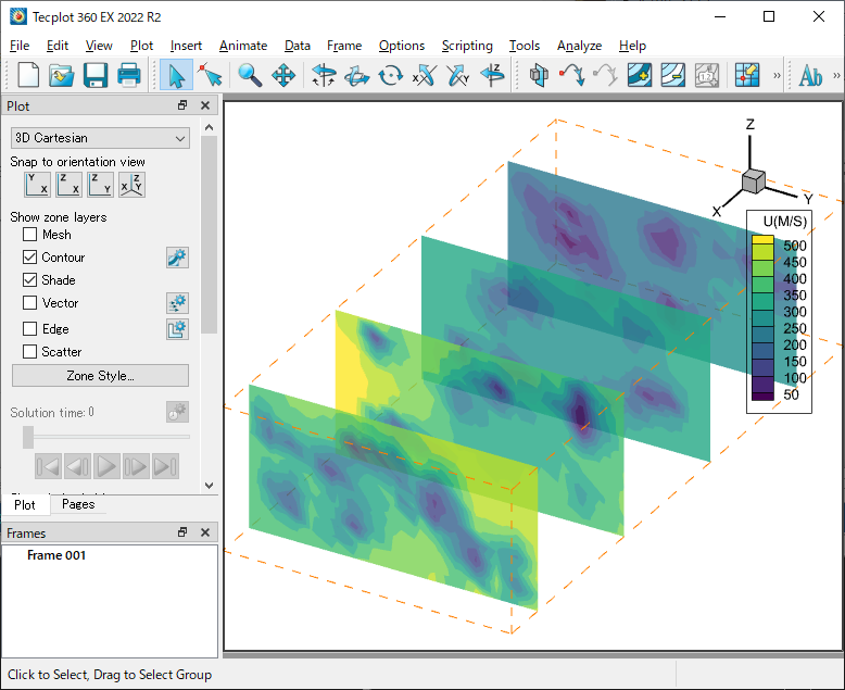
Tecplot の examples\SimpleData ディレクトリにあるプロットファイル DuctFlow.plt を読み込みます。スライスを有効にしてスライスオブジェクトを取得します。スライスの透明度を有効にします。等間隔の４つのスライスを設定します。スライスの X Velocity に関する等高線を有効にします。得られた内容を PNG 画像にエクスポートします。

• 例

  from os import path
  import tecplot as tp
  from tecplot.constant import SliceSurface, ContourType
  
  # Run this script with "-c" to connect to  Tecplot 360 on port 7600
  # To enable connections in Tecplot 360, click on:
  #   "Scripting" -> "PyTecplot  Connections..." -> "Accept connections"
  import sys
  if '-c' in sys.argv:
      tp.session.connect()
  
  examples_dir = tp.session.tecplot_examples_directory()
  datafile = path.join(examples_dir, 'SimpleData', 'DuctFlow.plt')
  dataset = tp.data.load_tecplot(datafile)
  
  plot = tp.active_frame().plot()
  plot.contour(0).variable = dataset.variable('U(M/S)')
  plot.show_contour = True
  
  # Turn on slice and get handle to slice object
  plot.show_slices = True
  slice_0 = plot.slice(0)
  
  # Turn on slice translucency
  slice_0.effects.use_translucency = True
  slice_0.effects.surface_translucency = 20
  
  # Setup 4 evenly spaced slices
  slice_0.show_primary_slice = False
  slice_0.show_start_and_end_slices = True
  slice_0.show_intermediate_slices = True
  slice_0.start_position = (-.21, .05, .025)
  slice_0.end_position = (1.342, .95, .475)
  slice_0.num_intermediate_slices = 2
  
  # Turn on contours of X Velocity on the slice
  slice_0.contour.show = True
  plot.contour(0).levels.reset_to_nice()
  
  tp.export.save_png('slices.png', 600, supersample=3) 

• 実行結果
  

 

14_isosurface.py

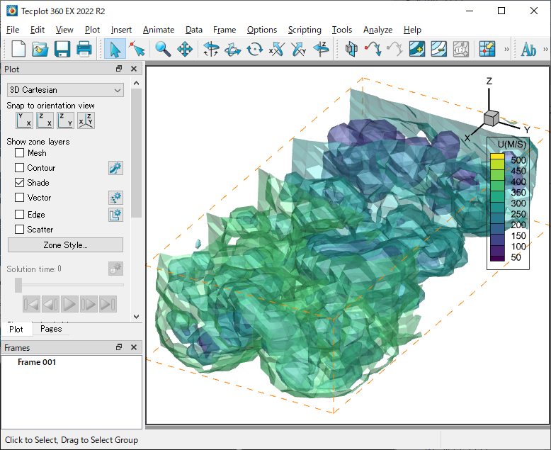
Tecplot の examples\SimpleData ディレクトリにあるプロットファイル DuctFlow.plt を読み込みます。等値面の各種表示を設定します。表示内容を PNG 画像に出力します。

• スクリプト：

  from os import path
  
  import tecplot as tp
  from tecplot.constant import LightingEffect, IsoSurfaceSelection
  
  # Run this script with "-c" to connect to  Tecplot 360 on port 7600
  # To enable connections in Tecplot 360, click on:
  #   "Scripting" -> "PyTecplot  Connections..." -> "Accept connections"
  import sys
  if '-c' in sys.argv:
      tp.session.connect()
  
  examples_dir = tp.session.tecplot_examples_directory()
  datafile = path.join(examples_dir, 'SimpleData', 'DuctFlow.plt')
  dataset = tp.data.load_tecplot(datafile)
  
  plot = tp.active_frame().plot()
  plot.contour(0).variable = dataset.variable('U(M/S)')
  
  plot.show_isosurfaces = True
  
  iso = plot.isosurface(0)
  
  iso.isosurface_selection = IsoSurfaceSelection.ThreeSpecificValues
  iso.isosurface_values = (135.674706817, 264.930212259, 394.185717702)
  
  iso.shade.use_lighting_effect = True
  iso.effects.lighting_effect = LightingEffect.Paneled
  iso.contour.show = True
  iso.effects.use_translucency = True
  iso.effects.surface_translucency = 50
  
  # ensure consistent output between interactive  (connected) and batch
  plot.contour(0).levels.reset_to_nice()
  
  tp.export.save_png('isosurface_example.png', 600, supersample=3) 

• 実行結果
  

 

15_wing_mach_iso.py

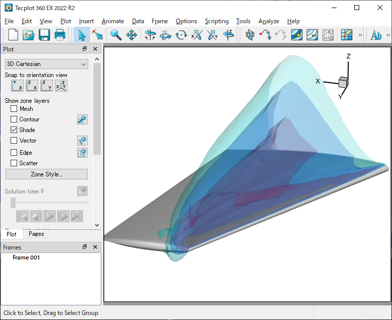
Tecplot の examples\OneraM6wing ディレクトリにあるプロットファイル OneraM6_SU2_RANS.plt を現在アクティブなフレームに読み込みます。Contour Levels の最初のグループと一致する Isosurface を設定します。Isosurface レイヤーの定義を設定します。半透明の指定を有効にします。複数の Isosurface を表示します。得られた内容を PNG 画像にエクスポートします。

• スクリプト：

  import tecplot
  from tecplot.constant import *
  import os
  
  # Run this script with "-c" to connect to  Tecplot 360 on port 7600
  # To enable connections in Tecplot 360, click on:
  #   "Scripting" -> "PyTecplot  Connections..." -> "Accept connections"
  import sys
  if '-c' in sys.argv:
      tecplot.session.connect()
  
  examples_dir = tecplot.session.tecplot_examples_directory()
  datafile = os.path.join(examples_dir, 'OneraM6wing', 'OneraM6_SU2_RANS.plt')
  ds = tecplot.data.load_tecplot(datafile)
  
  frame = tecplot.active_frame()
  plot = frame.plot()
  
  # Set Isosurface to match Contour Levels of the first  group.
  iso = plot.isosurface(0)
  iso.isosurface_selection = IsoSurfaceSelection.AllContourLevels
  cont = plot.contour(0)
  iso.definition_contour_group = cont
  cont.colormap_name = 'Magma'
  
  # Setup definition Isosurface layers
  cont.variable = ds.variable('Mach')
  cont.levels.reset_levels( [.95,1.0,1.1,1.4])
  print(list(cont.levels))
  
  # Turn on Translucency
  iso.effects.use_translucency = True
  iso.effects.surface_translucency = 80
  
  # Turn on Isosurfaces
  plot.show_isosurfaces = True
  iso.show = True
  
  cont.legend.show = False
  
  view = plot.view
  view.psi = 65.777
  view.theta = 166.415
  view.alpha = -1.05394
  view.position = (-23.92541680486183, 101.8931504712126, 47.04269529295333)
  view.width = 1.3844
  
  tecplot.export.save_png("wing_iso.png",width=600, supersample=3) 

• 実行結果
  

 

17_streamtrace_line.py

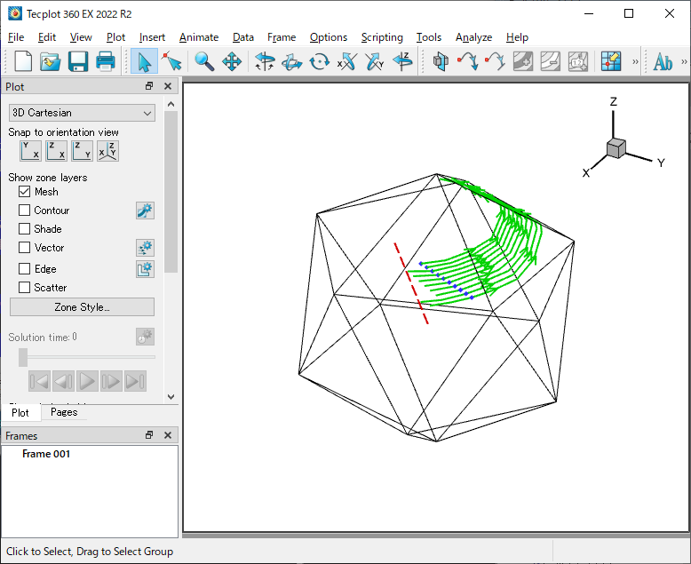
Tecplot の examples\SimpleData ディレクトリにあるプロットファイル Eddy.plt を現在アクティブなフレームに読み込みます。プロットタイプに 3D Cartesian を指定して、表示する 3D プロットと streamtrace の各種属性を指定します。streamtrace の終了ラインを赤の破線に指定します。マーカーを青の菱形に指定します。Surface Line の streamtrace を 追加します。得られた内容を PNG 画像にエクスポートします。

• スクリプト：

  import os
  import tecplot
  from tecplot.constant import *
  from tecplot.plot import Cartesian3DFieldPlot
  
  # Run this script with "-c" to connect to  Tecplot 360 on port 7600
  # To enable connections in Tecplot 360, click on:
  #   "Scripting" -> "PyTecplot  Connections..." -> "Accept connections"
  import sys
  if '-c' in sys.argv:
      tecplot.session.connect()
  
  examples_dir = tecplot.session.tecplot_examples_directory()
  datafile = os.path.join(examples_dir, 'SimpleData', 'Eddy.plt')
  dataset = tecplot.data.load_tecplot(datafile)
  
  frame = tecplot.active_frame()
  frame.plot_type = tecplot.constant.PlotType.Cartesian3D
  
  plot = frame.plot()
  plot.fieldmap(0).surfaces.surfaces_to_plot = SurfacesToPlot.BoundaryFaces
  plot.show_mesh = True
  plot.show_shade = False
  
  plot.vector.u_variable_index = 4
  plot.vector.v_variable_index = 5
  plot.vector.w_variable_index = 6
  plot.show_streamtraces = True
  
  streamtrace = plot.streamtraces
  streamtrace.color = Color.Green
  
  streamtrace.show_paths = True
  streamtrace.show_arrows = True
  streamtrace.arrowhead_size = 3
  streamtrace.step_size = .25
  streamtrace.line_thickness = .4
  streamtrace.max_steps = 10
  
  # Streamtraces termination line:
  streamtrace.set_termination_line([(-25.521, 39.866),
                                     (-4.618, -11.180)])
  
  # Streamtraces will stop at the termination line when  active
  streamtrace.termination_line.active = True
  
  # We can also show the termination line itself
  streamtrace.termination_line.show = True
  streamtrace.termination_line.color = Color.Red
  streamtrace.termination_line.line_thickness = 0.4
  streamtrace.termination_line.line_pattern = LinePattern.LongDash
  
  # Markers
  streamtrace.show_markers = True
  streamtrace.marker_color = Color.Blue
  streamtrace.marker_symbol_type = SymbolType.Geometry
  streamtrace.marker_symbol().shape = GeomShape.Diamond
  
  # Add surface line streamtraces
  streamtrace.add_rake(start_position=(45.49, 15.32, 59.1),
                       end_position=(48.89, 53.2, 47.6),
                       stream_type=Streamtrace.SurfaceLine)
  
  tecplot.export.save_png('streamtrace_line_example.png', 600, supersample=3) 

• 実行結果
  

 

19_streamtrace_2D.py

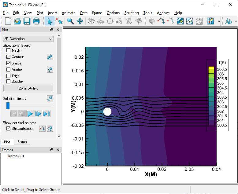
Tecplot の examples\SimpleData ディレクトリにあるプロットファイル VortexShedding.plt を現在アクティブなフレームに 2D Cartesian として読み込みます。ベクトルと背景に表示する等高線の属性を設定します。Streamtrace を追加し、そのスタイルを指定します。得られた内容を PNG 画像にエクスポートします。

• スクリプト：

  import tecplot
  from tecplot.constant import *
  import os
  
  # Run this script with "-c" to connect to  Tecplot 360 on port 7600
  # To enable connections in Tecplot 360, click on:
  #   "Scripting" -> "PyTecplot  Connections..." -> "Accept connections"
  import sys
  if '-c' in sys.argv:
      tecplot.session.connect()
  
  examples_dir = tecplot.session.tecplot_examples_directory()
  datafile = os.path.join(examples_dir, 'SimpleData', 'VortexShedding.plt')
  dataset = tecplot.data.load_tecplot(datafile)
  
  frame = tecplot.active_frame()
  frame.plot_type = tecplot.constant.PlotType.Cartesian2D
  
  # Setup up vectors and background contour
  plot = frame.plot()
  plot.vector.u_variable = dataset.variable('U(M/S)')
  plot.vector.v_variable = dataset.variable('V(M/S)')
  plot.contour(0).variable = dataset.variable('T(K)')
  plot.show_streamtraces = True
  plot.show_contour = True
  plot.fieldmap(0).contour.show = True
  
  # Add streamtraces and set streamtrace style
  streamtraces = plot.streamtraces
  streamtraces.add_rake(start_position=(-0.003, 0.005),
                        end_position=(-0.003, -0.005),
                        stream_type=Streamtrace.TwoDLine,
                        num_seed_points=10)
  
  streamtraces.show_arrows = False
  streamtraces.line_thickness = .4
  
  plot.axes.y_axis.min = -0.02
  plot.axes.y_axis.max = 0.02
  plot.axes.x_axis.min = -0.008
  plot.axes.x_axis.max = 0.04
  
  tecplot.export.save_png('streamtrace_2D.png', 600, supersample=3) 

• 実行結果
  

 

20_legend_line.py

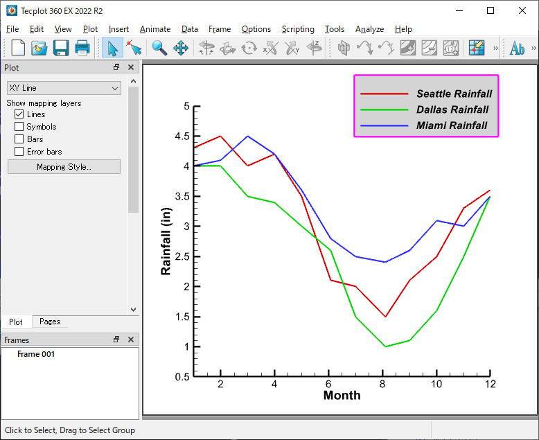
Tecplot の examples\SimpleData ディレクトリにあるデータファイル Rainfall.dat を現在アクティブなフレームに XY Line プロットとして読み込みます。Y 軸のラベルと範囲を指定します。凡例の表示を有効にし、各種属性を設定します。得られた内容を PNG 画像にエクスポートします。

• スクリプト：

  import os
  
  import tecplot
  from tecplot.constant import *
  
  # Run this script with "-c" to connect to  Tecplot 360 on port 7600
  # To enable connections in Tecplot 360, click on:
  #   "Scripting" -> "PyTecplot  Connections..." -> "Accept connections"
  import sys
  if '-c' in sys.argv:
      tecplot.session.connect()
  
  examples_dir = tecplot.session.tecplot_examples_directory()
  datafile = os.path.join(examples_dir, 'SimpleData', 'Rainfall.dat')
  dataset = tecplot.data.load_tecplot(datafile)
  
  frame = tecplot.active_frame()
  plot = frame.plot()
  frame.plot_type = tecplot.constant.PlotType.XYLine
  
  for i in range(3):
      plot.linemap(i).show = True
      plot.linemap(i).line.line_thickness = .4
  
  y_axis = plot.axes.y_axis(0)
  y_axis.title.title_mode = AxisTitleMode.UseText
  y_axis.title.text = 'Rainfall (in)'
  y_axis.fit_range_to_nice()
  
  legend = plot.legend
  legend.show = True
  legend.box.box_type = TextBox.Filled
  legend.box.color = Color.Purple
  legend.box.fill_color = Color.LightGrey
  legend.box.line_thickness = .4
  legend.box.margin = 5
  
  legend.anchor_alignment = AnchorAlignment.MiddleRight
  legend.row_spacing = 1.5
  legend.show_text = True
  legend.font.typeface = 'Arial'
  legend.font.italic = True
  
  legend.text_color = Color.Black
  legend.position = (90, 88)
  
  tecplot.export.save_png('legend_line.png', 600, supersample=3) 

• 実行結果
  

 

22_view_3D.py

Tecplot の examples\SimpleData ディレクトリにあるプロットファイル F18.plt を現在アクティブなフレームに 3D Cartesian プロットとして読み込みます。表示するサイズや角度を指定します。得られた内容を PNG 画像にエクスポートします。

• スクリプト：

  import tecplot
  import os
  from tecplot.constant import *
  
  # Run this script with "-c" to connect to  Tecplot 360 on port 7600
  # To enable connections in Tecplot 360, click on:
  #   "Scripting" -> "PyTecplot  Connections..." -> "Accept connections"
  import sys
  if '-c' in sys.argv:
      tecplot.session.connect()
  
  examples_dir = tecplot.session.tecplot_examples_directory()
  infile = os.path.join(examples_dir, 'SimpleData', 'F18.plt')
  ds = tecplot.data.load_tecplot(infile)
  plot = tecplot.active_frame().plot(PlotType.Cartesian3D)
  plot.activate()
  plot.view.width = 17.5
  plot.view.alpha = 0
  plot.view.theta = 125
  plot.view.psi = 65
  plot.view.position = (-100, 80, 65)
  
  tecplot.export.save_png('3D_view.png', 600, supersample=3) 

• 実行結果
  

 

24_frame_position.py

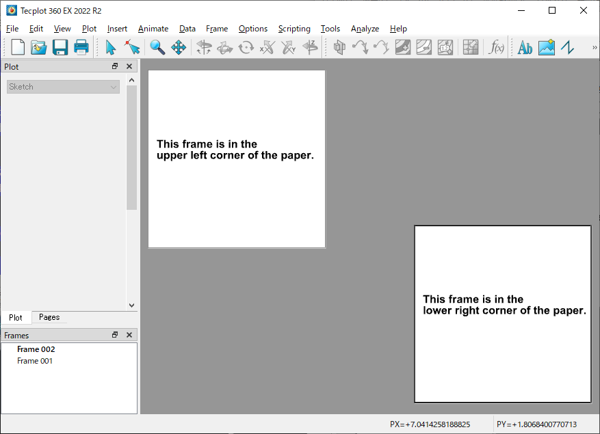
サイズと位置を指定した２つのフレームを生成し、それぞれにテキストとその位置とサイズを指定します。得られた結果を PNG 画像に出力します。

• スクリプト：

  import tecplot as tp
  from tecplot.constant import ExportRegion
  
  # Run this script with "-c" to connect to  Tecplot 360 on port 7600
  # To enable connections in Tecplot 360, click on:
  #   "Scripting" -> "PyTecplot  Connections..." -> "Accept connections"
  import sys
  if '-c' in sys.argv:
      tp.session.connect()
      tp.new_layout()
  
  frame1 = tp.active_frame()
  frame1.add_text('This frame is in the\nupper left corner of the paper.',
                  position=(5, 50), size=18)
  frame1.width = 4
  frame1.height = 4
  frame1.position = (.5, .5)
  
  frame2 = tp.active_page().add_frame()
  frame2.width = 4
  frame2.height = 4
  frame2.add_text('This frame is in the\nlower right corner of the paper.',
                  position=(5, 50), size=18)
  frame2.position = (6.5, 4)
  
  tp.export.save_png('frame_position.png', 600, supersample=3,
                     region=ExportRegion.WorkArea) 

• 実行結果
  

 

filledlines.py

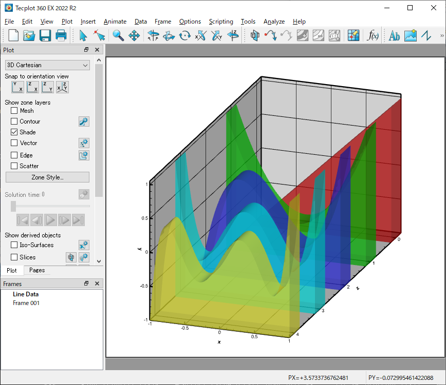
(x, y) であらわされる複数のラインプロットを 3D ボリュームとしてプロットします。

パラメータ：

• x (array)：x 軸方向の値の配列
• *yy (array)：x 値のそれぞれに対応する y 値の単一または複数の配列。この配列は "x" と同じ長さである必要があります。
• z (2-tuple)：各ラインプロットの z 方向の幅を (min, max) であらわすデータ対。
• y0 (float)：y 値の基底
• colors (tecplot.plot.ContourGroup or array of Colors)：コンターグループは、与えられた範囲の値を使ってラインプロット毎に色付けします。範囲を指定しない場合は、"tecplot.constant.color" で指定されたカラーが各ラインプロットに繰り返し使用されます。デフォルトでは、プロットの最初のコンターグループが使用されます。
• Name (str)：フレームの名称です。これを使ってフレーム呼び出したり作成したりします。ゾーンを呼び出したり作成したりするのにも使います。この文字列で始まるゾーン以外はデータセットから削除します。
• page (tecplot.layout.Page)：フレームを追加したり取得するページです。デフォルトでは、アクティブなページが使用されます。
• ルジャンドル (Legedre) 多項式を複数プロットする例：

import numpy as np
from numpy.polynomial import legendre 
import tecplot as tp 
x = np.linspace(-1., 1., 100) 
yy = [legendre.Legendre(([0] * i) + [1])(x) for i in range(1, 6)] 
plot = plot_filled_lines_3d(x, *yy, y0=-1.) 
tp.save_png('line_data.png') 

• もし、ページを開いていなければ、指定した名称でフレームを取得または作成します。フレームにデータセットがあればそれを使い、無ければ作成します。yy の値にもとづいて "{name} {i}" という名称のゾーンを作成または変更します。形状に変更があればゾーンを再度作成します。Tecplot にプッシュする配列を用意します。ゾーンにデータを代入します。前回の実行で生成された余計なゾーンを削除します。ラインの各ゾーンを表示するようプロットを調整します。軸変数、コンター変数を設定し、凡例を非表示に設定します。Shade カラーを使って各ゾーンを色分けします。コンターの範囲全体のコンター値を使って各ゾーンを色分けします。軸、コンター、半透明を有効にします。方向軸を非表示にします。サーフェスを有効にして、半透明を調整します。ビューを設定します。軸の範囲を設定します。z 軸の目盛り間隔を調整します。ビューにあわせて若干ズームアウトします。サンプルデータを生成します (直交多項式の系列)。Tecplot のカラーパレットを使って各ラインに陰影をつけます。または、color に None を指定してプロットのコンターカラーの値を使用します。

• コマンドライン実行例

  py filledlines.py -c

• スクリプト：

  from collections.abc import Iterable
  import itertools as it
  
  import tecplot as tp
  from tecplot.constant import AxisMode, Color, PlotType, SurfacesToPlot
  
  def plot_filled_lines_3d(x, *yy, z=(-0.5, 0.5), y0=0, colors=None,
                            name='Line Data', page=None):
      """Plot a series of  lines in (x, y) as 3D volumes.
  
      Parameters:
          x (array): Values along  the x-axis
          *yy (arrays): One or more  arrays of y-values for each x value. These
              must be the  same length as ``x``.
          z (2-tuple): (min, max)  around the z-coordinate for each line.
          y0 (float): Base y-value.
          colors  (tecplot.plot.ContourGroup or array of Colors): The contour
              group will  color each line using the full range if given.
              Otherwise,  colors obtained from the enumeration
               ``tecplot.constant.Color`` will be cycled through for each line.
              The first  contour group of the plot will be used by default.
          name (str): Name of the  frame that will be fetched or created. Also
              used to  fetch or create zones by name. Any other zones that start
              with this  string will be deleted from the dataset.
          page (tecplot.layout.Page):  Page on which to add or get the frame. The
              active page  will be used by default.
  
      Example plotting some Legedre  polynomials::
  
          import numpy as np
          from numpy.polynomial  import legendre
  
          import tecplot as tp
  
          x = np.linspace(-1., 1.,  100)
          yy =  [legendre.Legendre(([0] * i) + [1])(x) for i in range(1, 6)]
          plot =  plot_filled_lines_3d(x, *yy, y0=-1.)
           tp.save_png('line_data.png')
      """
      if page is None:
          page = tp.active_page()
  
      # get or create a frame with the given  name
      frame = page.frame(name)
      if frame is None:
          frame = page.add_frame()
          frame.name = name
  
      # use existing dataset on frame or  create it
      if frame.has_dataset:
          ds = frame.dataset
          vnames = ds.variable_names
          for vname in ['x', 'y', 'z', 's']:
              if vname not in vnames:
                  ds.add_variable(vname)
      else:
          ds = frame.create_dataset(name,  ['x', 'y', 'z', 's'])
  
      # create or modify zones named  "{name} {i}" based on the values in yy
      x = np.asarray(x, dtype=float)
      for i, y in enumerate(yy):
          shape = (len(x), 2, 2)
          zname = '{name} {i}'.format(name=name, i=i)
          zn = ds.zone(zname)
  
          # recreate zone if shape  has changed
          if zn is None or zn.dimensions != shape:
              new_zn = ds.add_ordered_zone(zname, shape)
              if zn:
                  ds.delete_zones(zn)
              zn = new_zn
  
          # prepare arrays to be  pushed into tecplot
          y1 = np.array([float(y0), 1.])
          z1 = np.asarray(z, dtype=float) + i
          Z, Y, X = np.meshgrid(z1, y1, x, indexing='ij')
          Y[:,1,:] = y
  
          # fill zone with data
          zn.values('x')[:] = X
          zn.values('y')[:] = Y
          zn.values('z')[:] = Z
          zn.values('s')[:] = np.full(Z.size, i / ((len(yy) - 1) or 1))
  
      # remove any extra zones from a  previous run
      zones_to_delete = []
      while True:
          i = i + 1
          zn = ds.zone('{name} {i}'.format(name=name, i=i))
          if zn is None:
              break
          zones_to_delete.append(zn)
      if zones_to_delete:
          ds.delete_zones(*zones_to_delete)
  
      # adjust plot to show the line zones
      plot = frame.plot(PlotType.Cartesian3D)
      plot.activate()
  
      # set axes variables, contour variable,  hide legend
      plot.axes.x_axis.variable = ds.variable('x')
  
      plot.axes.y_axis.variable = ds.variable('y')
      plot.axes.z_axis.variable = ds.variable('z')
  
      if isinstance(colors, Iterable):
          # color each zone by  shade color
          plot.show_contour = False
          plot.show_shade = True
          for zn, col in zip(ds.zones(name + ' *'), it.cycle(colors)):
              plot.fieldmap(zn).shade.color = Color(col)
      else:
          # color each zone by  contour values over the whole contour range
          if colors is None:
              contour = plot.contour(0)
          plot.show_contour = True
          plot.show_shade = False
          contour.variable = ds.variable('s')
          contour.legend.show = False
          contour.levels.reset_levels(np.linspace(0, 1, 256))
  
      # turn on axes, contour and  translucency. hide orientation axes
      plot.axes.x_axis.show = True
      plot.axes.y_axis.show = True
      plot.axes.z_axis.show = True
      plot.use_translucency = True
      plot.axes.orientation_axis.show = False
  
      # turn on surfaces and adjust  translucency
      for zn in ds.zones('Line Data*'):
          fmap = plot.fieldmap(zn)
          fmap.show = True
          fmap.surfaces.surfaces_to_plot = SurfacesToPlot.BoundaryFaces
          fmap.effects.surface_translucency = 50
  
      # set the view
      plot.view.psi = 0
      plot.view.theta = 0
      plot.view.alpha = 0
      plot.view.rotate_axes(20, (1, 0, 0))
      plot.view.rotate_axes(-20, (0, 1, 0))
  
      # set axes limits
      ax = plot.axes
      ax.axis_mode = AxisMode.Independent
      ax.x_axis.min = min(x)
      ax.x_axis.max = max(x)
      ax.y_axis.min = y0
      ax.y_axis.max = 1.05 * ds.variable('y').max()
      ax.z_axis.min = z[0]
      ax.z_axis.max = z[1] + (len(yy) - 1)
  
      # adjust tick spacing for z-axis
      ax.z_axis.ticks.auto_spacing = False
      ax.z_axis.ticks.spacing = 1
  
      # fit the view and then zoom out  slightly
      plot.view.fit()
      plot.view.width *= 1.05
  
      return plot
  
  if __name__ == '__main__':
      import sys
      import numpy as np
      from numpy import polynomial as poly
  
      from tecplot.constant import Color
  
      if '-c' in sys.argv:
          tp.session.connect()
  
      # some sample data (orthogonal  polynomial series)
      x = np.linspace(-1., 1., 100)
      yy = [poly.legendre.Legendre(([0] * i) + [1])(x)
            for i in range(1, 6)]
  
      # use tecplot color palette to shade  each line
      # alternatively, set colors to None to  use the
      # plot's contour color values.
      colors = [Color(i + 1) for i in range(len(yy))]
      plot = plot_filled_lines_3d(x, *yy, y0=-1, colors=colors)
  
      if '-c' not in sys.argv:
          tp.save_png('line_data.png')

• 実行結果
  

 

Forces_Moments_VS_Span.py

関数の内容：

• 力とモーメントを計算する (３つの手法。詳細は https://kb.tecplot.com/2018/02/23/calculating-aerodynamic-forces-moments/ 参照)
• 指定した方向に n 個のサーフェスのスライスを作成して抽出する。
• スライスの集合に対してスカラー積分を実行する
• 積分の結果を距離に対してプロットする

各サーフェスの力とモーメントを計算する：

• 手法：pressureOnly, pressureShear, pressureVelocity
• pressure, shear, velocity, dynamicVisc: フィールド変数の名称
• surface_zones: 積分を実行するサーフェスのゾーン

サーフェスの単位ベクトルの法線を計算します。Tecplot の方程式ツールで使用する文字列を手法に応じて定義します。指定した方向に min から max まで等間隔に配置された numPts 個のスライスを定義し、抽出します。スライスをゾーンに抽出します。スライスゾーンを名称で取得します。この部分は PyTecplot 1.4 移行で動作します。上記の2行は slice_zones = sl.extract() に置き換えることができます。sliceZnes をループし、各スライスの力とモーメントの積分を実行します (スカラー積分、変数は手法によって変わります)。([dir, irNormalized, fxNr, fyNr, fzNr, mxNr, myNr, mzNr]*Nslices array) を返します。力とモーメントの変数を取得します。返された配列に方向と積分値を入力します。方向を正規化します。

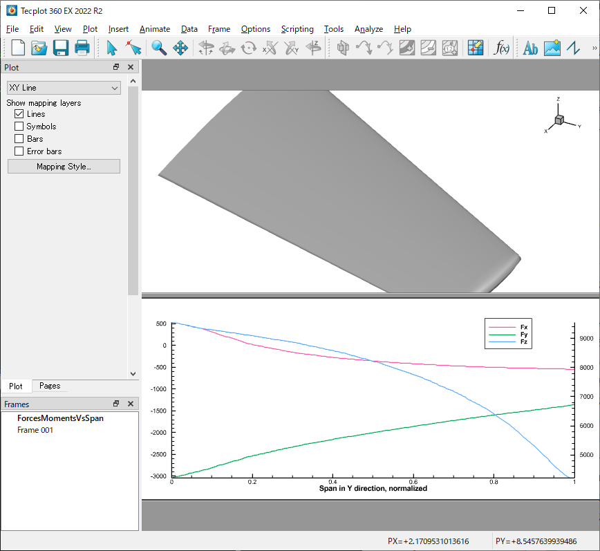
Forces VS Span のプロットを実行します。プロットタイプを変更したり、スタイルシートを読み込んでみてください。新規ページまたは新規フレームにプロットします。力とモーメントの行列を格納するデータセットを作成します。プロットを定義します。既存のラインマップを削除します。力とモーメントを成分とするラインマップを作成します。凡例と軸を設定します。

メインの処理：このスクリプトは ForcesAndMoments.py に定義された関数の使用法を説明するものです。使用するデータセットは、ONERA M6 wing です。このデータは Tecplot のインストールディレクトリの /examples/OneraM6wing にあります。

正しいフィールド変数の設定するには：Pressure and Velocity を実行するときは、変数の番号と変数の名称が正しいことを確認します。なお、ここでの変数は 1 で始まる点に注意してください。

力とモーメントを計算します。時間を短縮するため計算はサーフェスゾーンに限定します。翼に沿って nPts 個のスライスを作成します。各スライスの力とモーメントを統合します。力とモーメントをスパンに対してプロットします。

• コマンドライン実行例：

  py Forces_Moments_VS_Span.py

• 例

  import numpy as np
  import os.path
  import sys
  import tecplot as tp
  from tecplot.constant import Color, PlotType, SliceSource, SliceSurface, ValueLocation
  
  '''
  A set of functions to:
  - calculate forces and moments (3 methods, for  details see:
       https://kb.tecplot.com/2018/02/23/calculating-aerodynamic-forces-moments/)
  - create and extract n surface slices in a given  direction
  - perform a scalar integration on a set of slices
  - plots the integration results against the distance
  '''
  
  def calcForcesMoments(method, surface_zones, pressure, shear=["","",""], velocity=["","",""], dynamicVisc=""):
      """Computes forces and  moments on a surface:
      - method: pressureOnly, pressureShear,  pressureVelocity
      - pressure, shear, velocity,  dynamicVisc: the field variables names
      - surface_zones: the surface zone(s)  for the integration to be performed
      """
  
      #Computes the unit vector normal to the  surface
      tp.macro.execute_extended_command(command_processor_id='CFDAnalyzer4',
          command="Calculate  Function='GRIDKUNITNORMAL' Normalization='None'"\
              +" ValueLocation='CellCentered'  CalculateOnDemand='F'"\
                  +" UseMorePointsForFEGradientCalculations='F'")
          
      #Defines the string used in Tecplot's  equations tool depending on the method
      eq = list()
      if method == "Pressure":
          eq += ['{px} = -{'+'{}'.format(pressure)+'}* {X Grid K Unit  Normal}']
          eq += ['{py} = -{'+'{}'.format(pressure)+'}* {Y Grid K Unit  Normal}']
          eq += ['{pz} = -{'+'{}'.format(pressure)+'}* {Z Grid K Unit  Normal}']
          eq += ['{mx} = Y * {pz} - Z * {py}']
          eq += ['{my} = Z * {px} - X * {pz}']
          eq += ['{mz} = X * {py} - Y * {px}']
      elif method == "Pressure  and Shear":
          eq += ['{taux} = {'+'{}'.format(shear[0])+'}- {X Grid K Unit Normal} *{'\
              +'{}'.format(pressure)+'}']
          eq += ['{tauy} = {'+'{}'.format(shear[1])+'}- {Y Grid K Unit Normal} *{'\
              +'{}'.format(pressure)+'}']
          eq += ['{tauz} = {'+'{}'.format(shear[2])+'}- {Z Grid K Unit Normal} *{'\
              +'{}'.format(pressure)+'}']
          eq += ['{mx} = Y * {tauz} - Z * {tauy}']
          eq += ['{my} = Z * {taux} - X * {tauz}']
          eq += ['{mz} = X * {tauy} - Y * {taux}']
      elif method == "Pressure  and Velocity":
          tp.macro.execute_extended_command(command_processor_id='CFDAnalyzer4',
              command="Calculate Function='VELOCITYGRADIENT'  Normalization='None'"\
                  +" ValueLocation='Nodal'  CalculateOnDemand='F'"\
                      +"  UseMorePointsForFEGradientCalculations='F'")
          eq += ['{D} = {dUdX} + {dVdY} + {dWdZ}']
          eq += ['{T11} = {'+'{}'.format(dynamicVisc)+'} * (2 * {dUdX} - 2/3 * {D}) -{'\
              +'{}'.format(pressure)+'}']
          eq += ['{T12} = {'+'{}'.format(dynamicVisc)+'} * ({dVdX} + {dUdY})']
          eq += ['{T13} = {'+'{}'.format(dynamicVisc)+'} * ({dWdX} + {dUdZ})']
          eq += ['{T22} = {'+'{}'.format(dynamicVisc)+'} * (2 * {dVdY} - 2/3 * {D}) -{'\
              +'{}'.format(pressure)+'}']
          eq += ['{T23} = {'+'{}'.format(dynamicVisc)+'} * ({dVdZ} + {dWdY})']
          eq += ['{T33} = {'+'{}'.format(dynamicVisc)+'} * (2 * {dWdZ} - 2/3 * {D}) -{'\
              +'{}'.format(pressure)+'}']
          eq += ['{taux} = {T11} * {X Grid K Unit  Normal} + {T12} * {Y Grid K Unit Normal}'\
              +' + {T13} * {Z Grid K Unit Normal}']
          eq += ['{tauy} = {T12} * {X Grid K Unit  Normal} + {T22} * {Y Grid K Unit Normal}'\
              +' + {T23} * {Z Grid K Unit Normal}']
          eq += ['{tauz} = {T13} * {X Grid K Unit  Normal} + {T23} * {Y Grid K Unit Normal}'\
              +' + {T33} * {Z Grid K Unit Normal}']
          eq += ['{mx} = Y * {tauz} - Z * {tauy}']
          eq += ['{my} = Z * {taux} - X * {tauz}']
          eq += ['{mz} = X * {tauy} - Y * {taux}']
  
      for e in eq: #do the computation only on the zone(s) of interest
          tp.data.operate.execute_equation(e,zones=surface_zones,value_location=ValueLocation.CellCentered)
  
  def createSlices(numPts, direction, minPos, maxPos):
      """
      Defines and extracts numPts slices 
      equally spaced from min to max
      in the given direction
      """
  
      p=tp.active_frame().plot()
      ds = tp.active_frame().dataset
  
      p.show_slices=False
      sl=p.slice(0)
      sl.show_primary_slice=False
      sl.show_start_and_end_slices=True
      sl.slice_source=SliceSource.SurfaceZones
  
      if direction=="X":
          sl.orientation=SliceSurface.XPlanes
          sl.start_position=(minPos,0,0)
          sl.end_position=(maxPos,0,0)
      elif direction=="Y":
          sl.orientation=SliceSurface.YPlanes
          sl.start_position=(0,minPos,0)
          sl.end_position=(0,maxPos,0)
      elif direction=="Z":
          sl.orientation=SliceSurface.ZPlanes
          sl.start_position=(0,0,minPos)
          sl.end_position=(0,0,maxPos)
      else:
          print ("{} is not a valid direction (X,Y,Z) for the planes  creation.".format(direction))
      sl.show_intermediate_slices=True
      sl.num_intermediate_slices=numPts-2
  
      #Extract the slices to zones
      sl.show=True
      
      sl.extract()
      slice_zones = list(ds.zones("Slice*")) # Get slice zones by name
  
      # This should work in PyTecplot 1.4+   and can replace the above 2 lines 
      # slice_zones = sl.extract()
  
      return slice_zones
  
  def intForcesMoments(sliceZnes,method, direction):
      """
      Loops over the sliceZnes and performs  an integration of Forces and moments
      for each slice (Scalar integrals,  variables are depending on the method).
      Returns a ([dir,  dirNormalized,fxNr,fyNr,fzNr,mxNr,myNr,mzNr]*Nslices array) 
      """
      #direction, norm_direction,  fx,fy,fz,mx,my,mz
      forcesMoments=np.zeros((8,len(sliceZnes))) 
      
      ds = sliceZnes[0].dataset
      fr = ds.frame
      #Retrieves Forces and Moments variables
      xAxisNr=ds.variable(direction).index
      if method == "Pressure":
          fxNr=ds.variable('px').index
          fyNr=ds.variable('py').index
          fzNr=ds.variable('pz').index
      else:
          fxNr=ds.variable('taux').index
          fyNr=ds.variable('tauy').index
          fzNr=ds.variable('tauz').index
      mxNr=ds.variable('mx').index
      myNr=ds.variable('my').index
      mzNr=ds.variable('mz').index
  
      #Populates the returned array with the  direction and integrated values
      for i,slice_zone in enumerate(sliceZnes):
          forcesMoments[(0,i)]= slice_zone.values(xAxisNr)[0]
          for j,var_index in enumerate([fxNr,fyNr,fzNr,mxNr,myNr,mzNr]):
              intCmde=("Integrate  ["+"{}".format(slice_zone.index + 1)+"]  VariableOption='Scalar'"\
                  + " XOrigin=0 YOrigin=0  ZOrigin=0"\
                  +" ScalarVar=" + "{}".format(var_index+1)\
                  + " Absolute='F'  ExcludeBlanked='F' XVariable=1 YVariable=2 ZVariable=3 "\
                  + "IntegrateOver='Cells'  IntegrateBy='Zones'"\
                  + "IRange={MIN =1 MAX = 0 SKIP =  1}"\
                  + " JRange={MIN =1 MAX = 0 SKIP  = 1}"\
                  + " KRange={MIN =1 MAX = 0 SKIP  = 1}"\
                  + " PlotResults='F'  PlotAs='Result' TimeMin=0 TimeMax=0")
              tp.macro.execute_extended_command(command_processor_id='CFDAnalyzer4',
                  command=intCmde)
              integrated_result = float(fr.aux_data['CFDA.INTEGRATION_TOTAL'])
              forcesMoments[(j+2,i)] = integrated_result
              slice_zone.aux_data[ds.variable(var_index).name] = integrated_result
  
      #Normalized direction:
      forcesMoments[1]=(forcesMoments[0]-forcesMoments[0].min())/(forcesMoments[0].max()-forcesMoments[0].min())
  
      return (forcesMoments)
  
  def forcesMomentsVsSpan(forcesMoments, direction, normalized, newPage):
      """Performs the plot of  Forces VS Span.
      Feel free to modify the plot type or  load a stylesheet."""
      
      #Plot either on a new page or on a new  frame
      if newPage == True:
          tp.add_page()
          tp.active_page().name='ForcesMomentsVsSpan'
          fr = tp.active_frame()
      else:
          fr  = tp.active_page().add_frame()
          tp.macro.execute_extended_command(command_processor_id='Multi Frame Manager',
              command='TILEFRAMESHORIZ')
      fr.name='ForcesMomentsVsSpan'
  
      #Creates a dataset to host the forces  and moments matrix
      ds2 = fr.create_dataset('ForcesMomentsSpan',
          ['{}'.format(direction), 'Span in {} direction, normalized'.format(direction),
          'Fx','Fy','Fz', 'Mx', 'My', 'Mz'])
      zne=ds2.add_ordered_zone('Forces  and Moments',(len(forcesMoments[0])))
      for v in range(8):
          zne.values(v)[:] = forcesMoments[v].ravel()
  
      #Defines the plot
      fr.plot_type=PlotType.XYLine
      p = fr.plot()
  
      #Delete existing linemaps
      nLm=range(p.num_linemaps)
      for lm in nLm:
          p.delete_linemaps(0)
  
      #Create linemaps for each force and  moment component
      for lm in range(6):
          p.add_linemap()
          if normalized==False:
              p.linemap(lm).x_variable_index=0
          else:
              p.linemap(lm).x_variable_index=1
          p.linemap(lm).y_variable_index=lm+2
          p.linemap(lm).name='&DV&'
          p.linemap(lm).line.line_thickness=0.4
      p.linemap(2).y_axis_index=1 #Fz to be put on a  second Y-axis
      for lm in range(3,6):        #Do not show moments by default
          p.linemap(lm).show=False
      p.linemap(0).line.color=Color.Custom31
      p.linemap(1).line.color=Color.Custom28
      p.linemap(2).line.color=Color.Custom29
      p.view.fit()
  
      #Legend and Axis setup
      p.legend.show = True
      p.legend.position = (80, 90)
      p.axes.y_axis(0).title.offset=9
      p.axes.y_axis(1).title.offset=9
  
  '''
  Main
  This script illustrate how to use the functions  defined in ForcesAndMoments.py
  The dataset used is the ONERA M6 wing, that can be  found in:
  Tecplot's installation directory/examples/OneraM6wing
  '''
  
  #Slices Parameters:
  nPts=200
  direction="Y"
  minPos=0.05
  maxPos=1.15
  
  #Integration parameters:
  mode = "Pressure and Velocity"
  #mode = "Pressure"
  #mode = "Pressure and Shear"
  pressure_var_name="Pressure"
  sh=["Wall shear-1","Wall  shear-2","Wall shear-3"]
  dVi="SA Turbulent Eddy Viscosity" #"Turbulent Viscosity"
  
  #ForcesVSSpan parameters
  normalized=True
  newPage=False
  
  tp.session.connect()
  #tp.macro.execute_command("$!LoadAddon  'tecutiltools_combinezones'")
  
  #Loading the data
  tp.new_layout()
  examples_dir = tp.session.tecplot_examples_directory()
  datafile = os.path.join(examples_dir, 'OneraM6wing', 'OneraM6_SU2_RANS.plt')
  ds = tp.data.load_tecplot(datafile)
  fr=tp.active_frame()
  
  #setting the correct field variables
  #
  # TODO - Make sure that the variable numbers and variable names
  #  are correct when doing Pressure and  Velocity!!!
  #  NOTE - the variable numbers here are 1-based
  #
  if mode == "Pressure and  Velocity":
      tp.macro.execute_extended_command(command_processor_id='CFDAnalyzer4',
          command="SetFieldVariables  ConvectionVarsAreMomentum='T'"\
              +" UVar=5 VVar=6 WVar=7 ID1='Pressure' Variable1=10  ID2='Density' Variable2=4")
  
  #calculates the forces and moments, limit the  calculation to the surface zones to save time
  surface_zones = [z for z in ds.zones() if z.rank == 2]
  calcForcesMoments(mode,surface_zones,pressure_var_name,shear=sh,dynamicVisc=dVi)
  
  with tp.session.suspend():
      #Creating nPts slices along the wing
      slice_zones = createSlices(nPts,direction,minPos,maxPos)
  
  with tp.session.suspend():
      #Integrates the forces and moments on  each slice
      forcesMoments=intForcesMoments(slice_zones,mode,direction)
  
  with tp.session.suspend():
      #Plots the forces and moments VS span
      forcesMomentsVsSpan(forcesMoments, direction, normalized, newPage)
  
  #Delete the extracted slices
  #ds.delete_zones(s)

• 実行結果
  

 

Histogram.py

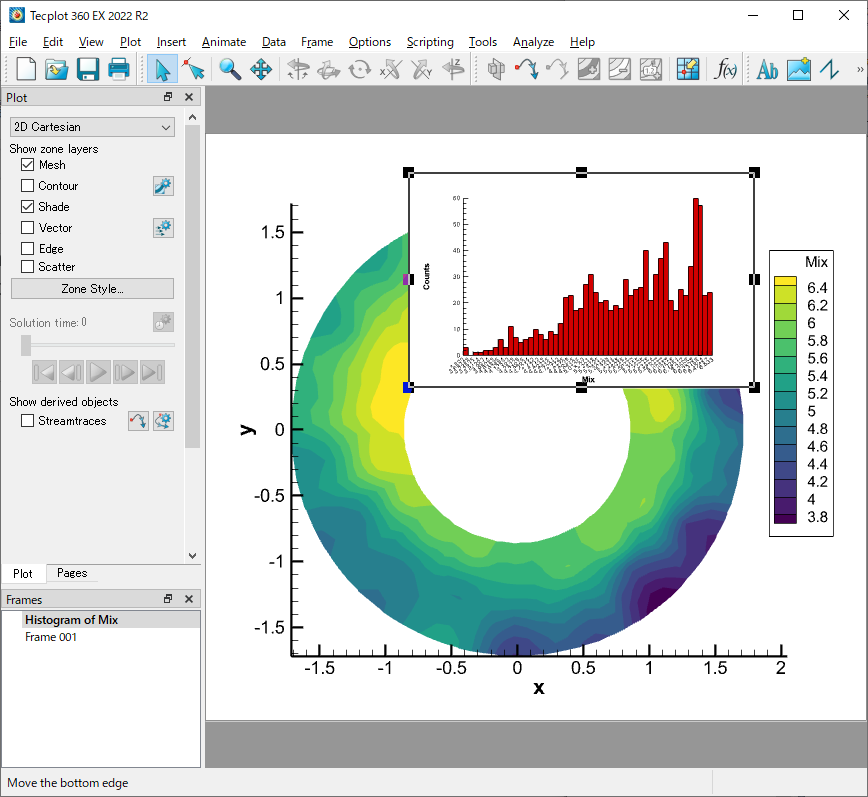
事前にプロット (例：CircularContour.plt) を開き、変数名を確認しておきます (例：Mix)。プロットを開いた状態で、以下の２つの引数を付けて実行します。

• コマンドライン構文：

  py Histogram.py <変数名> <ビンの数>

  コマンドライン実行例：

  py Histogram.py Mix 50

ヒストグラムの結果をあらわすフレームとデータセットを作成します。FE - Quad タイプのゾーンを作成し、各セルでビン数をあらわします。結果をあらわすプロットの各種スタイルを設定します。フィールドマップは１つだけになります。ビューポートを縮小して軸タイトルの場所を確保します。

• スクリプト：

  import tecplot as tp
  import numpy as np
  from tecplot.constant import *
  
  
  def plot_histogram(histogram, var_name):
      bins = histogram[0]
      edges = histogram[1]
  
      # Create a new frame and dataset to  hold the histogram results
      frame = tp.active_page().add_frame()
      ds = frame.create_dataset("Histogram of "+var_name, [var_name, "Counts"])
      frame.name = "Histogram  of {}".format(var_name)
  
      # Create a FE-Quad zone, where each  cell represents a bin
      zone = ds.add_fe_zone(ZoneType.FEQuad, "Histogram  of "+var_name, 4*len(bins), len(bins))
      xvals = []
      yvals = []
      connectivity = []
      for i,count in enumerate(bins):
          xvals.extend([edges[i], edges[i+1], edges[i+1], edges[i]])
          yvals.extend([0,0,count,count])
          connectivity.append([i*4, i*4+1, i*4+2, i*4+3])
      zone.values(0)[:] = xvals
      zone.values(1)[:] = yvals
      zone.nodemap[:] = connectivity
  
      # Setup the plot style to present the  results
      plot = frame.plot(tp.constant.PlotType.Cartesian2D)
      plot.activate()
      plot.axes.axis_mode = tp.constant.AxisMode.Independent
      plot.view.fit()
      x_axis = plot.axes.x_axis
      x_axis.ticks.auto_spacing = False
      x_axis.ticks.spacing_anchor = edges[0]
      x_axis.ticks.spacing = abs(edges[1] - edges[0])
      plot.show_mesh = True
      plot.show_shade = True
  
      # There will only be one fieldmap...
      for fmap in plot.fieldmaps():
          fmap.shade.color = tp.constant.Color.Red
  
      plot.axes.y_axis.title.offset = 10 
      plot.axes.y_axis.title.show = True
      plot.axes.x_axis.title.show = True
      plot.axes.x_axis.title.offset = 10 
  
      plot.axes.x_axis.tick_labels.offset = 1.5
      plot.axes.x_axis.tick_labels.angle = 35
      plot.axes.x_axis.tick_labels.show = True
      plot.axes.x_axis.ticks.minor_num_ticks = 0
  
      # Reduce the viewport make room for the  axis titles
      plot.axes.viewport.bottom=15
      plot.axes.viewport.left=16
  
      return plot
  
  def hist(var, bins = 5, zones = None):
      if not zones:
          zones = var.dataset.zones()
      zones = list(zones)
      all_values = np.array([])
      for z in zones:
          values = z.values(var).as_numpy_array()
          all_values = np.append(all_values, values)
      h = np.histogram(all_values, bins)
      return h
  
  if __name__ == "__main__":
      import argparse
      parser = argparse.ArgumentParser(description="Computes and  plots a histogram of a given variable.")
      parser.add_argument("varname", help="Name of the variable for which to compute the  histogram")
      parser.add_argument("bins", help="Number of bins in the histogram", type=int)
      args = parser.parse_args()
      tp.session.connect()
      with tp.session.suspend():
          dataset = tp.active_frame().dataset
          var_name = args.varname
          variable = dataset.variable(var_name)
          bins = args.bins
          zones = dataset.zones()
          h = hist(variable, bins, zones)
          plot = plot_histogram(h, variable.name) 

• 実行結果
  

 

UniformVectorViaGeom.py

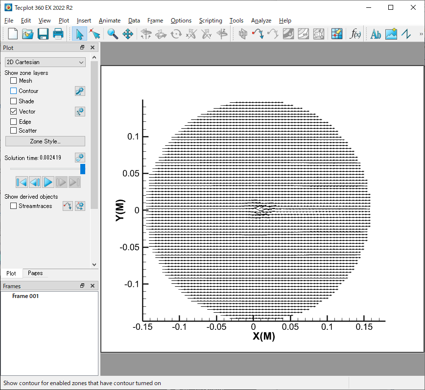
データセット VortexShedding.plt を読み込みます。（※スクリプト内のサンプルデータ (VortexShedding.plt) のパスは環境にあわせて変更してください。）

• コマンドライン実行例

  py UniformVectorViaGeom.py

• スクリプト：

  import tecplot as tp
  from tecplot.exception import *
  from tecplot.constant import *
  
  # Uncomment the following line to connect to a  running instance of Tecplot 360:
  tp.session.connect()
  
  tp.macro.execute_command("""$!ReadDataSet   '\"C:\\Program  Files\\Tecplot\\Tecplot 360 EX 2022  R2\\examples\\SimpleData\\VortexShedding.plt\" '
      ReadDataOption = New
      ResetStyle = Yes
      VarLoadMode = ByName
      AssignStrandIDs = Yes
      VarNameList = '\"X(M)\" \"Y(M)\" \"U(M/S)\" \"V(M/S)\" \"W(M/S)\" \"P(N/M2)\" \"T(K)\" \"R(KG/M3)\"'""")
  tp.macro.execute_command("""$!Pick  SetMouseMode
      MouseMode = Select""")
  
  cmd = """$!AttachGeom
      PositionCoordsys = FRAME
      RawData
      1
  """
  idxs = ""
  count = 0
  for i in range(10, 100, 1):
      for j in range(10, 100, 1):
          idxs += str(i) + ' ' + str(j) + '\n'
          count += 1
  # print (count)
  cmd += str(count) + '\n' + idxs
  print(cmd)
  tp.macro.execute_command(cmd)
  
  tp.macro.execute_command("""$!Pick  AddAll
      SELECTGEOMS=YES""")
  tp.macro.execute_command("""$!ExtractFromGeom
      ExtractLinePointsOnly = Yes
      IncludeDistanceVar = No
      NumPts = 200
      ExtractToFile = No""")
  tp.macro.execute_command("""$!Pick  Clear""")
  
  tp.active_frame().plot().fieldmap(0).vector.show = False
  tp.active_frame().plot(PlotType.Cartesian2D).vector.u_variable_index = 2
  tp.active_frame().plot(PlotType.Cartesian2D).vector.v_variable_index = 3
  tp.active_frame().plot().show_vector = True
  tp.active_frame().plot().fieldmap(1).vector.tangent_only = True
  tp.active_frame().plot().fieldmap(1).vector.tangent_only = False 

• 実行結果
  

 

plot_max_over_time.py

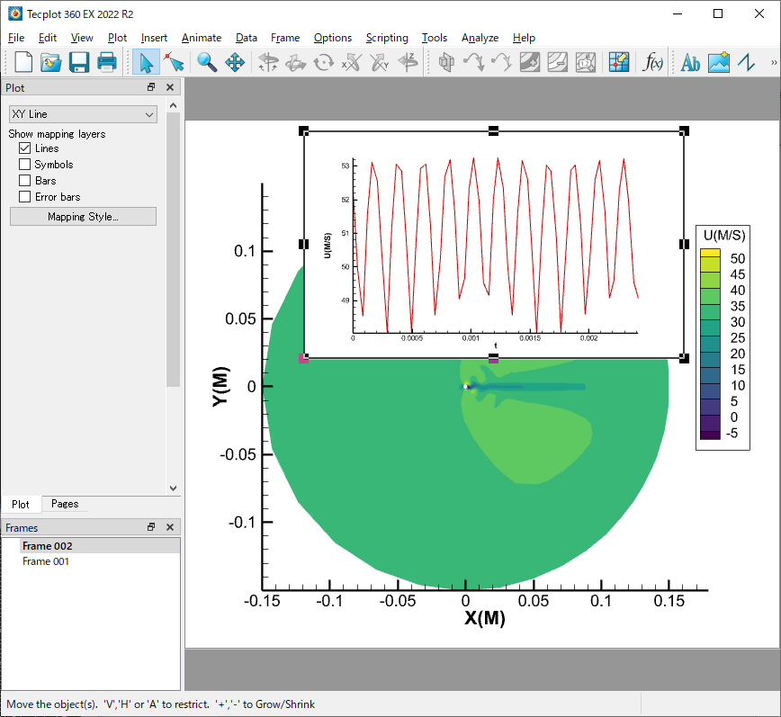
各ゾーンの最大値を折れ線グラフであらわします。スクリプトを実行するには、事前に Example フォルダの VortexShedding.plt を Tecplot に開いておいてください。詳しくは下記ビデオの 6:00 以降をご覧ください。

https://www.tecplot.com/2020/01/10/webinar-ask-the-expert-about-tecplot-360/

実行時間を短縮するために、インターフェースを一時停止します。フレームを新規作成し、抽出したそれぞれの最大値をプロット作成に使用します。

• コマンドライン実行例

  py plot_max_over_time.py

• スクリプト：

  """Plots the maximums for one  zone through time
  
  Description
  -----------
  This connected-mode script creates a line graph of  the maximum values from a zone
  over time, as seen in this Ask the Expert video (at  ~6:00):
  https://www.tecplot.com/2020/01/10/webinar-ask-the-expert-about-tecplot-360/
  
  Usage:
      > python plot_max_over_time.py
  
  For example data, see the link above, or the  VortexShedding.plt file found in the 
  examples directory in the Tecplot 360 installation  folder.
  """
  
  import tecplot as tp
  from tecplot.constant import *
  tp.session.connect() #connect to a  live running instance of Tecplot 360
  
  # Suspend the interface to speed up execution time
  with tp.session.suspend():
      dataset = tp.active_frame().dataset
      values = []
      var_name = 'U(M/S)'
      for z in dataset.zones():
          values.append((z.solution_time, z.values(var_name).max()))
  
      # Create a new frame and stuff the  extracted values into it for plotting
      new_frame = tp.active_page().add_frame()
      ds = new_frame.create_dataset('Max {} over time'.format(var_name), ['t',var_name])
      zone = ds.add_ordered_zone('Max {} over  time'.format(var_name), len(values))
      zone.values('t')[:] = [v[0] for v in values]
      zone.values(var_name)[:] = [v[1] for v in values]
      new_frame.plot(PlotType.XYLine).activate() 

• 実行結果
  

 

pyqt5_execute_macro_command.py

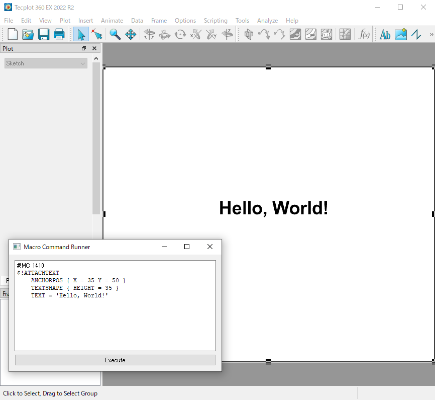
Tecplot マクロコマンドを *.mcr ファイルとして保存しなくとも記述して実行できる GUI を作成します。

必要なモジュール：PyQt5 (クロスプラットフォームアプリケーションフレームワーク Qt を Python で使うためのモジュールです) https://pypi.org/project/PyQt5/

• インストール法：

  py -m pip install "PyQt5"

スクリプトを実行するには、まず Tecplot 360 ユーザー インターフェイスの Scripting > PyTecplot Connections... ダイアログで Accept connections をクリックします。

• コマンドライン実行例

  py -O pyqt5_execute_macro_command.py

スクリプトを実行すると、Tecplot マクロコマンドを受け入れることができる PyQt5 GUI が起動します。 GUIで Execute を押すとマクロコマンドが一時ファイルに保存されて実行されるため、自分でファイルを作成する手間が省けます。

• スクリプト：

  """
  Creates a graphical user interface (GUI) that allows  you to enter and execute Tecplot macro
  commands without having to create a *.mcr file.
  usage:
      > python -O pyqt5_execute_macro_command.py
  Necessary modules
  -----------------
  tecplot
      The PyTecplot package
      https://pypi.org/project/pytecplot/
  PyQt5
      Python bindings for the Qt cross  platform application toolkit
      https://pypi.org/project/PyQt5/
  Description
  -----------
  To run this script, first "Accept  connections" in the Tecplot 360 user interface via
  the "Scripting>PyTecplot Connections..."  dialog
  Running this script will launch a PyQt5 GUI that can  accept Tecplot macro
  commands. When "Execute" is pressed in the  GUI, the macro commands are saved to a
  temporary file, then executed, saving you the effort  of creating a file yourself.
  """
  
  import sys
  import os
  import tempfile
  import tecplot as tp
  from PyQt5 import QtWidgets, QtGui
  
  class ExecuteMacroCommand(QtWidgets.QWidget):
      def __init__(self):
          super(ExecuteMacroCommand, self).__init__()
          self.initUI()
  
      def initUI(self):
          self.macro_command_textEdit = QtWidgets.QTextEdit()
          self.macro_command_textEdit.setPlainText("#!MC 1410")
  
          addExecuteMacroCommand_Button = QtWidgets.QPushButton("Execute")
          addExecuteMacroCommand_Button.clicked.connect(self.execute_macro_command_CB)
  
          vbox = QtWidgets.QVBoxLayout()
          vbox.addWidget(self.macro_command_textEdit)
          vbox.addWidget(addExecuteMacroCommand_Button)
  
          self.setLayout(vbox)
  
          self.setGeometry(300, 300, 800, 600)
          self.setWindowTitle('Macro  Command Runner')
          self.show()
  
      def execute_macro_command_CB(self, *a):
          cmd = self.macro_command_textEdit.toPlainText()
          try: 
              temp_file = tempfile.NamedTemporaryFile(delete=False, suffix=".mcr")
              temp_file.write(cmd.encode('utf8'))
              temp_file.flush()
              tp.macro.execute_file(temp_file.name)
          except Exception as e:
              error_dialog = QtWidgets.QMessageBox()
              error_dialog.setWindowTitle("Error")
              if str(e):
                  error_dialog.setText("Error: {}".format(str(e)))
              else:
                  error_dialog.setText("Error:\nNo error details available. ")
              error_dialog.exec_()
          finally:
              temp_file.close()
              os.unlink(temp_file.name)
  
  if __name__ == '__main__':
      try:
          tp.session.connect()
          app = QtWidgets.QApplication(sys.argv)
          ex = ExecuteMacroCommand()
          res = app.exec_()
          sys.exit(res)
      except Exception as e:
          log("Error")
          log(str(e)) 

• 実行結果